6 Four Examples of statistical models
This chapter treats in some detail four main examples of statistical models. These are all parametric models, and a central computational challenge is to fit the models to data via (penalized) likelihood maximization. The actual optimization algorithms and implementations are the topics of Chapters 7, 8 and 9. The focus of this chapter is on the structure of the statistical models themselves to provide the necessary background for the later chapters.
Statistical models come in many varieties, and the abstract mathematical definition of a statistical model is as a parametrized families of probability distributions. To say anything of interest, we need more structure such as structure on the parameter set, properties of the parametrized distributions, and properties of the mapping from the parameter set to the distributions. For any specific model we have all that structure but often also an overwhelming amount of irrelevant details that will be more distracting than clarifying. The intention is that the four examples treated will illustrate the breath of statistical models that share important structures without getting lost in abstractions.
In the first section we introduce the key idea of a parametrized statistical model and give some simple examples. We give the definition of the (log-)likelihood function and touch on the phenomenon that computationally important properties of the log-likelihood function may depend on the chosen parametrization. In the subsequent sections we cover multinomial models, regression models, mixture models and random effects models as our four main examples.
6.1 Parametrized models and the likelihood
In all our examples we will consider a parameter set \(\Theta \subseteq \mathbb{R}^p\) and a parametrized family of probability distributions on a common sample space denoted \(\mathcal{Y}\). The distribution corresponding to \(\theta \in \Theta\) is assumed to have a density \(f_{\theta}\) (w.r.t. a \(\theta\)-independent reference measure).
In many applications, the sample space is a product space
\[ \mathcal{Y} = \mathcal{Y}_1 \times \ldots \times \mathcal{Y}_N \]
corresponding to observations \(y_1 \in \mathcal{Y}_1, \ldots, y_N \in \mathcal{Y}_N\). We will in this case be interested in modeling the observations as independent but not necessarily identically distributed. Thus the joint density is a product
\[ f_{\theta}(y_1, \ldots, y_N) = \prod_{i=1}^N f_{i,\theta}(y_i). \ \]
Note that the density, \(f_{i,\theta}\), is a density for a probability distribution on \(\mathcal{Y}_i\), and that all these densities are parametrized by the same parameter \(\theta \in \Theta\), but due to the \(i\)-index they may differ. If all the densities are equal, data is modeled as i.i.d.
The likelihood function is, for fixed data \(y = (y_1, \ldots, y_N)\), the function
\[ \mathcal{L}(\theta) = \prod_{i=1}^N f_{i,\theta}(y_i), \]
as a function of the parameter \(\theta\). The log-likelihood function is
\[ \ell(\theta) = \log (\mathcal{L}(\theta)) = \sum_{i=1}^N \log(f_{i,\theta}(y_i)), \]
and the negative log-likelihood function is \(-\ell\). In practice, we will minimize the negative log-likelihood function over the parameter set to find the model within the parametrized family of distributions that best fits the data. The resulting parameter estimate is known as the maximum-likelihood estimate.
Example 6.1 Poisson distributions with sample space \(\mathcal{Y} = \mathbb{N}_0 = \{0, 1, 2, \ldots \}\) are typically used to model non-negative integer counts. The Poisson distributions are parametrized by the mean parameter \(\mu > 0\), and the density is given by the point probabilities
\[ f_{\mu}(y)= e^{-\mu} \frac{\mu^y}{y!}. \]
The parameter space is thus \(\Theta = (0, \infty)\).
With i.i.d. observations \(y_1, \ldots, y_N\) the negative log-likelihood is given by
\[ - \ell(\mu) = \sum_{i=1}^N \left( \mu - y_i \log(\mu) + \log(y!) \right) = n \mu - \log(\mu) \sum_{i=1}^N y_i + n \log(y!). \]
For this model we can find an analytic expression for the maximum-likelihood estimate. By differentiating twice we see that
\[\begin{align*} - \ell'(\mu) & = n - \frac{1}{\mu} \sum_{i=1}^N y_i \\ - \ell''(\mu) & = \frac{1}{\mu^2} \sum_{i=1}^N y_i \geq 0 \end{align*}\]
Since the second derivative is non-negative, the negative log-likelihood is convex, and a solution to \(- \ell'(\mu) = 0\) will be a global minimizer. We see that if \(\sum_{i=1}^N y_i > 0\), the unique solution to this equation is
\[ \hat{\mu} =\frac{1}{n} \sum_{i=1}^N y_i \]
and this is thus the maximum-likelihood estimate.
If \(\sum_{i=1}^N y_i = 0\) (which is equivalent to \(y_1 = y_2 = \ldots = y_N = 0\)) there is no minimizer in the open parameter set \((0, \infty)\). We could argue that \(\hat{\mu} = 0\) in this case, if we extended the parameter space to include \(0\).
Note that the (negative) log-likelihood depends on data only though the data transformation \(\sum_{i=1}^N y_i\). We call this sum a since it is sufficient for the computation of the log-likelihood and the maximum-likelihood estimate.
The Poisson model with i.i.d. data is so simple that we can minimize the negative log-likelihood analytically. This is not possible for many other statistical models as the following example will illustrate.
Example 6.2 Recall the von Mises distributions on the sample space \(\mathcal{Y} = (-\pi, \pi]\), which were introduced in Section 1.2.1. They were introduced as a parametrized family of probability distributions with density
\[ f_{\theta}(y) = \frac{1}{\varphi(\theta)} e^{\theta_1 \cos(y) + \theta_2 \sin(y)} \]
for \(\theta = (\theta_1, \theta_2) \in \mathbb{R}^2\). That is, \(\Theta = \mathbb{R}^2\). The function
\[\varphi(\theta) = \int_{-\pi}^{\pi} e^{\theta_1 \cos(u) + \theta_2 \sin(u)} \mathrm{d}u < \infty\]
for \(\theta \in \Theta\) can be expressed in terms of a modified Bessel function, but it cannot be expressed in terms of elementary functions.
An alternative parametrization was also introduced in Section 1.2.1 in terms of polar coordinates given by the reparametrization map
\[(\kappa, \mu) \mapsto \theta = \kappa \left(\begin{array}{c} \cos(\mu) \\ \sin(\mu) \end{array}\right)\]
that maps \([0,\infty) \times (-\pi, \pi]\) onto \(\Theta\). This alternative \((\kappa, \mu)\)-parametrization has several problems. First, the \(\mu\) parameter is not identifiable if \(\kappa = 0\), which is reflected by the fact that the reparametrization is not a one-to-one map. Second, the parameter space is not open, which can be quite a nuisance for, e.g., maxmimum-likelihood estimation. We could circumvent these problems by restricting attention to \((\kappa, \mu) \in (0,\infty) \times (-\pi, \pi)\), but we would then miss some of the distributions parametrized by \(\theta\)— notably the uniform distribution corresponding to \(\theta = 0\).
With observations \(y_1, \ldots, y_N\) the negative log-likelihood in the \(\theta\)-parametrization becomes
\[ - \ell(\theta) = \log \varphi(\theta) - \theta_1 \sum_{i=1}^N \cos(y_i) - \theta_2 \sum_{i=1}^N \sin(y_i). \]
This function can be shown to be convex. Moreover, with this parametrization the log-likelihood only depends on data through the two statistics \(\sum_{i=1}^N \cos(y_i)\) and \(\sum_{i=1}^N \sin(y_i)\), which are thus sufficient statistics. When minimizing the negative numerically log-likelihood, the sufficient statistics can be computed once upfront instead of repeatedly every time the negative log-likelihood is evaluated.
Using the \((\kappa, \mu)\)-parametrization the negative log-likelihood is
\[ - \ell(\kappa, \mu) = \log \varphi(\kappa (\cos(\mu), \sin(\mu))^T) - \kappa \sum_{i=1}^N \cos(y_i - \mu). \]
see also Section 1.2.1. This function is not necessarily convex, and without essentially reexpressing it in terms of the \(\theta\)-parametrization it does not reveal any sufficient statistics.
Irrespectively of the chosen parametrization, we will not be able to
find an analytic formula for the maximum-likelihood estimate. We have to
rely on numerical optimization procedures. When doing so, it can be
beneficial to use an appropriate parametrization, e.g., one where the
negative log-likelihood is convex and where computations of it and its
gradient can be implemented efficiently.
The example above with the von Mises distributions illustrates how the log-likelihood is specified in terms of the densities and data as a function of the parameters. The example also shows that the precise form of the log-likelihood depends on the specific parametrization. The parametrization determines, for instance, whether the negative log-likelihood is convex, and it can also reveal or hide whether there exist sufficient statistics.
Example 6.3 The family of Gaussian distributions on \(\mathbb{R}\) is most often parametrized by the mean \(\mu \in \mathbb{R}\) and variance \(\sigma^2 > 0\). The density for the \(\mathcal{N}(\mu, \sigma^2)\)-distribution is
\[\begin{align*} f_{\mu, \sigma^2}(y) & = \frac{1}{\sqrt{2\pi\sigma^2}}\exp\left(-\frac{(y - \mu)^2}{2\sigma^2}\right) \\ & = \frac{1}{\sqrt{\pi}} \exp\left(\frac{\mu}{\sigma^2} y - \frac{1}{2\sigma^2} y^2 - \frac{\mu^2}{2\sigma^2} - \frac{1}{2}\log (2\sigma^2) \right), \end{align*}\]
and the parameter space is \(\mathbb{R} \times (0, \infty)\).
Up to the factor \(1/{\sqrt{pi}}\), the negative log-likelihood with \(N\) observations is
\[ - \ell(\mu, \sigma) = \frac{\mu}{\sigma^2} \sum_{i=1}^N y_i - \frac{1}{2\sigma^2} \sum_{i=1}^N y^2_i - n \frac{\mu^2}{2\sigma^2} - n \frac{1}{2}\log (2\sigma^2). \]
We see that \(\sum_{i=1}^N y_i\) and \(\sum_{i=1}^N y_i^2\) constitute sufficient statistics. It is possible to show that the unique maximum-likelihood estimate (when at least two of the observations differ) equals
\[\begin{align*} \hat{\mu} & = \frac{1}{n} \sum_{i=1}^N y_i \\ \hat{\sigma}^2 & = \frac{1}{n} \sum_{i=1}^N (y_i - \hat{\mu})^2. \\ \end{align*}\]
It is fairly straightforward to show that \((\hat{\mu}, \hat{\sigma}^2) \in \mathbb{R} \times (0, \infty)\) is the unique stationary point, but the negative log-likelihood is not convex in the \((\mu, \sigma^2)\)-parametrization, which makes it a bit tricky to show that the solution above is, indeed, the global minimizer.
One possibility is to use the reparametrization
\[ \theta_1 = \frac{\mu}{\sigma^2} \quad \text{and} \quad \theta_2 = \frac{1}{2 \sigma^2}, \]
which gives
\[ - \ell(\theta_1, \theta_2) = \theta_1 \sum_{i=1}^N y_i - \theta_2 \sum_{i=1}^N y^2_i - n \frac{\theta_1^2}{4\theta_2} + n \frac{1}{2}\log (\theta_2). \]
This function is convex in \(\theta = (\theta_1, \theta_2)^T \in \mathbb{R} \times (0,\infty)\). If we choose to minimize \(- \ell\) in this parametrization, we can return to the mean and variance parameters via
\[\mu = \frac{\theta_1}{2\theta_2} \quad \text{and} \quad \sigma^2 = \frac{1}{2\theta_2}.\]
In all three examples above we found one parametrization where
- we could identify sufficient statistics
- and where the negative log-likelihood is convex
The examples are with its canonical parametrization leading to the two desirable properties above. It is far from all statistical models that are exponential families, but even the more complicated models are often build from simpler components that are, in fact, exponential families. We will in several cases take advantage of such an underlying exponential family structure of the components – even though we will avoid a full fledged treatment of exponential families, see Lauritzen (2023). For the implementation of computations and optimization algorithms, what matters most is the possibility to exploit sufficient statistics and convexity of the negative log-likelihood to yield fast computations and convergence guarantees of the algorithms.
6.2 Multinomial models
The multinomial model is the model of all probability distributions on a finite set \(\mathcal{Y} = \{1, \ldots, K\}\). The full model is parametrized by the simplex
\[\Delta_K = \left\{(p_1, \ldots, p_K)^T \in \mathbb{R}^K \ \Biggm| \ p_y \geq 0, \ \sum_{y=1}^K p_y = 1\right\}.\]
The distributions parametrized by the relative interior of \(\Delta_K\) can be reparametrized as
\[p_y = \frac{e^{\theta_y}}{\sum_{k=1}^K e^{\theta_l}} \in (0,1)\]
for \(\theta = (\theta_1, \ldots, \theta_K)^T \in \mathbb{R}^K.\) The entries of a probability vector \(p \in \Delta_K\) can then be expressed as
\[p_y = \frac{e^{t(y)^T \theta}}{\varphi(\theta)}\]
where \(t(y) = (\delta_{1y}, \ldots, \delta_{Ky})^T \in \mathbb{R}^{K}\) (where \(\delta_{ky} \in \{0, 1\}\) is the Kronecker delta being 1 if and only if \(k = y\)), and
\[\varphi(\theta) = \sum_{k=1}^K e^{\theta_l}.\]
With \(N\) i.i.d. observations from a multinomial distribution we find that the log-likelihood function is
\[\begin{align*} \ell(\theta) & = \sum_{i=1}^N \sum_{k=1}^K \delta_{k y_i} \log(p_k(\theta)) \\ & = \sum_{k=1}^K \underbrace{\sum_{i=1}^N \delta_{k y_i}}_{= N_k} \log(p_k(\theta)) \\ & = \sum_{k=1}^K N_k \log(p_k(\theta)) \\ & = \theta^T \mathbf{N} - N \log \left(\varphi(\theta) \right) \\ & = \theta^T \mathbf{N} - N \log \left(\sum_{k=1}^{K} e^{\theta_k} \right). \end{align*}\]
where \(\mathbf{N} = (N_1, \ldots, N_K)^T = \sum_{i=1}^N t(y_i) \in \mathbb{N}_0^K\) is the sufficient statistic, which is simply a tabulation of the times the different elements in \(\{1, \ldots, K\}\) were observed. The term \(\log \left(\varphi(\theta) \right)\) is a convex function, and since the other term is linear, \(- \ell\) is convex in the \(\theta\)-parametrization.
The distribution of the tabulated data, \(\mathbf{N}\), is a multinomial distribution with parameters \((N, p)\), and we often write \(\mathbf{N} \sim \textrm{Mult}(N, p)\).
We call the \(\theta\)-parametrization above with \(\theta \in \mathbb{R}^K\) the symmetric parametrization. Unfortunately, this parameter is not identifiable from the probability vector \(p\)—adding a constant to all entries of \(\theta\) will give the same probability vector. The lack of identifiability is traditionally fixed by setting \(\theta_K = 0\). This results in the parameter \(\theta = (\theta_1, \ldots, \theta_{K-1})^T \in \mathbb{R}^{K-1},\) in the sufficient statistic \(t(y) = (\delta_{1y}, \ldots, \delta_{(K-1)y})^T \in \mathbb{R}^{K-1}\), and
\[\varphi(\theta) = 1 + \sum_{k=1}^{K-1} e^{\theta_k}.\]
The category \(K\) is known as the reference category, and the parameter \(\theta_y\) now expresses the difference relative to the reference category:
\[p_y = \left\{\begin{array}{ll} \frac{e^{\theta_y}}{\varphi(\theta)} & \quad \text{if } y = 1, \ldots, K-1 \\ \frac{1}{\varphi(\theta)} & \quad \text{if } y = K. \end{array}\right.\]
We see that \(p_y = e^{\theta_y}p_K\) for \(y = 1, \ldots, K-1\), with the probability of the reference category \(K\) acting as a baseline probability, and the factor \(e^{\theta_y}\) acting as a multiplicative modification of this baseline. Moreover, the ratios
\[\frac{p_y}{p_k} = e^{\theta_y - \theta_k},\]
are independent of the chosen baseline. The log-likelihood becomes
\[\begin{align*} \ell(\theta) & = \theta^T \mathbf{N} - N \log \left(1 + \sum_{k=1}^{K - 1} e^{\theta_k} \right). \end{align*}\]
In the special case of \(K = 2\) the two elements \(\mathcal{Y}\) are often given other labels than \(1\) and \(2\). The most common labels are \(\{0, 1\}\) and \(\{-1, 1\}\). If we use the \(0\)-\(1\)-labels the convention is to use \(p_0\) as the baseline and thus
\[p_1 = \frac{e^{\theta}}{1 + e^{\theta}} = e^{\theta} p_0 = e^{\theta} (1 - p_1)\]
is parametrized by \(\theta \in \mathbb{R}\). As this function of \(\theta\) is known as the logistic function, this parametrization of the probability distributions on \(\{0,1\}\) is called the logistic model. From the above we see that
\[\theta = \log \frac{p_1}{1 - p_1}\]
is the log-odds.
If we use the \(\pm 1\)-labels, an alternative parametrization is
\[p_y = \frac{e^{y\theta}}{e^\theta + e^{-\theta}}\]
for \(\theta \in \mathbb{R}\) and \(y \in \{-1, 1\}\). This gives a symmetric treatment of the two labels while retaining the identifiability.
6.2.1 Peppered Moths
The color of the peppered moth (Birkemåler in Danish) is divided into three categories: black, mottled and light colored. Figure 6.1 shows examples of the color variation among individual moths. The peppered moth provided an early demonstration of evolution in the 19th century England, where the light colored moth was outnumbered by the dark colored variety. The dark color became dominant due to the increased pollution, where trees were darkened by soot, and had for that reason a selective advantage.
The color is the directly observable phenotype of the moth, while the genetics is a little more complicated. The color of the moth is primarily determined by one gene that occur in three different alleles denoted C, I and T. The alleles are ordered in terms of dominance as C > I > T. Moths with a genotype including C are dark. Moths with genotype TT are light colored. Moths with genotypes II and IT are mottled. Thus there a total of six different genotypes (CC, CI, CT, II, IT and TT) and three different phenotypes (black, mottled, light colored).

Figure 6.1: Examples of the color variation of the peppered moth.
If we sample \(N\) moths and classify them according to color we have a sample from a multinomial distribution with three categories. If we could observe the genotypes, we would have a sample from a multinomial distribution with six categories. To make matters a little more complicated, the multinomial probability vector is in either case determined by the allele frequencies, which we denote \(p_C\), \(p_I\), \(p_T\) with \(p_C + p_I + p_T = 1.\) According to the Hardy-Weinberg principle, the genotype frequencies are then
\[\begin{align*} p_{CC} &= p_C^2, \ p_{CI} = 2p_Cp_I, \ p_{CT} = 2p_Cp_T \\ p_{II} &= p_I^2, \ p_{IT} = 2p_Ip_T, \ p_{TT} = p_T^2. \end{align*}\]
The parametrization in terms of allele frequencies maps out a subset of the full parameter set for the multinomial distribution with six categories. If we could observe the genotypes, the multinomial log-likelihood, parametrized by allele frequencies, would be
\[\begin{align*} \ell(p_C, p_I) & = 2N_{CC} \log(p_C) + N_{CI} \log (2 p_C p_I) + N_{CT} \log(2 p_C p_I) + 2 N_{II} \log(p_I) \\ & \ \ + N_{IT} \log(2p_I p_T) + 2 N_{TT} \log(p_T) \\ & = 2N_{CC} \log(p_C) + N_{CI} \log (2 p_C p_I) + N_{CT} \log(2 p_C p_I) + 2 N_{II} \log(p_I) \\ & \ \ + N_{IT} \log(2p_I (1 - p_C - p_I)) + 2 N_{TT} \log(1 - p_C - p_I). \end{align*}\]
The log-likelihood is given in terms of the genotype counts and the two probability parameters \(p_C, p_I \geq 0\) with \(p_C + p_I \leq 1\). By differentiation, it is possible to find an analytic expression for the maximum-likelihood estimate, but we will postpone this exercise to Section 8.1.3, because collecting moths and determining their color will only identify their phenotype, not their genotype. Thus we observe \((N_C, N_T, N_I)\), where
\[N = \underbrace{N_{CC} + N_{CI} + N_{CT}}_{= N_C} + \underbrace{N_{IT} + N_{II}}_{=N_I} + \underbrace{N_{TT}}_{=N_T}.\]
For maximum-likelihood estimation of the parameters from the observation \((N_C, N_T, N_I)\) we need the likelihood in the marginal distribution of the observed variables.
It is useful to view the example with the peppered moths as an example of the general phenomenon of cell collapsing in a multinomial model. In general, let \(A_1 \cup \ldots \cup A_{K_0} = \{1, \ldots, K\}\) be a partition and let
\[M : \mathbb{N}_0^K \to \mathbb{N}_0^{K_0}\]
be the map given by
\[M((N_1, \ldots, N_K))_j = \sum_{k \in A_j} N_k.\]
If \(\mathbf{N} \sim \textrm{Mult}(N, p)\) with \(p = (p_1, \ldots, p_K)\) then
\[\mathbf{X} = M(\mathbf{N}) \sim \textrm{Mult}(N, M(p)).\]
With \(\psi \mapsto p(\psi)\) a parametrization of the cell probabilities, the log-likelihood under the collapsed multinomial model is generally
\[\begin{equation} \ell(\theta) = \sum_{j = 1}^{K_0} x_j \log (M(p(\psi))_j) = \sum_{j = 1}^{K_0} x_j \log \left(\sum_{k \in A_j} p_k(\psi)\right). \tag{6.1} \end{equation}\]
For the peppered Moths, \(K = 6\) corresponds to the six genotypes, \(K_0 = 3\) corrosponds to the three phenotypes, and the partition corresponding to the phenotypes is
\[\{1, 2, 3\} \cup \{4, 5\} \cup \{6\} = \{1, \ldots, 6\},\]
and
\[M(N_1, \ldots, N_6) = (N_1 + N_2 + N_3, N_4 + N_5, N_6).\]
In terms of the \(\psi = (p_C, p_I)\)-parametrization, \(p_T = 1 - p_C - p_I\) and
\[p = (p_C^2, 2p_Cp_I, 2p_Cp_T, p_I^2, 2p_Ip_T, p_T^2).\]
Hence
\[M(p) = (p_C^2 + 2p_Cp_I + 2p_Cp_T, p_I^2 +2p_Ip_T, p_T^2).\]
The log-likelihood equals
\[\begin{align} \ell(p_C, p_I) & = N_C \log(p_C^2 + 2p_Cp_I + 2p_Cp_T) + N_I \log(p_I^2 +2p_Ip_T) + N_T \log (p_T^2). \end{align}\]
We implement the log-likelihood in a very problem specific way below. The implementation includes a test of whether the parameter constraints are fulfilled, that is, whether \((p_C, p_I, P_t)\) is a probability vector. If the parameter constraints are violated the function returns the value \(+\infty\). It is fairly standard in optimization to encode constraints by letting the function return the value \(+\infty\) for parameters that do not fulfill the constraints.
# par = c(pC, pI), pT = 1 - pC - pI
# x is the data vector of counts of length 3
loglik <- function(par, x) {
  pT <- 1 - par[1] - par[2]

  if (par[1] > 1 || par[1] < 0 || par[2] > 1 || par[2] < 0 || pT < 0)
    return(Inf)

  PC <- par[1]^2 + 2 * par[1] * par[2] + 2 * par[1] * pT
  PI <- par[2]^2 + 2 * par[2] * pT
  PT <- pT^2
  # The function returns the negative log-likelihood
  - (x[1] * log(PC) + x[2] * log(PI) + x[3] * log(PT))
}
It is possible to use optim() in R with just this implementation to
compute the maximum-likelihood estimate of the allele parameters.
## $par
## [1] 0.07085 0.18872
##
## $value
## [1] 600.5
##
## $counts
## function gradient
##       71       NA
##
## $convergence
## [1] 0
##
## $message
## NULL
The optim() function uses an algorithm called Nelder-Mead
as the default algorithm, which relies on log-likelihood evaluations only. It
is slow but fairly robust. A bit of thought has to go into the initial
parameter choice, though.
Starting the algorithm at a boundary value, where the negative log-likelihood attains
the value \(\infty\), does not work.
## Error in optim(c(0, 0), loglik, x = c(85, 196, 341)): function
cannot be evaluated at initial parameters
The computations can beneficially be implemented in greater
generality. The function M() below implements cell collapsing
by adding up the entries of all cells belonging to the same
group as specified by the group argument.
The log-likelihood for multinomial cell collapsing is then implemented below
via M() and two problem specific arguments to
the loglik() function. One of these is a vector specifying
the grouping structure of the collapsing. The other is a function
that determines the
parametrization that maps the parameter that we optimize over to the
cell probabilities. In the implementation it is assumed
that this prob() function in addition encodes parameter constraints
by returning NULL if parameter constraints are violated.
loglik <- function(par, x, prob, group, ...) {
  p <- prob(par)
  if(is.null(p)) return(Inf)
  - sum(x * log(M(prob(par), group)))
}
The function prob() is implemented specifically for the peppered moth example
as follows.
prob_pep <- function(p) {
  p[3] <- 1 - p[1] - p[2]
  if (p[1] > 1 || p[1] < 0 || p[2] > 1 || p[2] < 0 || p[3] < 0)
    return(NULL)
  c(p[1]^2, 2 * p[1] * p[2], 2* p[1] * p[3],
    p[2]^2, 2 * p[2] * p[3], p[3]^2)
}
We test that the new implementation gives the same maximum-likelihood estimate as the problem specific implementation above.
## $par
## [1] 0.07085 0.18872
##
## $value
## [1] 600.5
##
## $counts
## function gradient
##       71       NA
##
## $convergence
## [1] 0
##
## $message
## NULL
Once we have found an estimate of the parameters, we can compute a prediction of the unobserved genotype counts from the phenotype counts using the conditional distribution of the genotypes given the phenotypes. This is straightforward as the conditional distribution of \(\mathbf{N}_{A_j} = (Y_k)_{k \in A_j}\) given \(\mathbf{X} = \mathbf{x}\) is also a multinomial distribution;
\[\mathbf{N}_{A_j} \mid \mathbf{X} = \mathbf{x} \sim \textrm{Mult}\left( x_j, \frac{p_{A_j}}{M(p)_j} \right).\]
The probability parameters are simply \(p\) restricted to \(A_j\) and renormalized to a probability vector. Observe that this gives
\[E (N_k \mid \mathbf{X} = \mathbf{x}) = \frac{x_j p_k}{M(p)_j}\]
for \(k \in A_j\). Using the estimated parameters and the M() function implemented
above, we can compute a prediction of the genotype counts as follows.
x <- c(85, 196, 341)
group <- c(1, 1, 1, 2, 2, 3)
p <- prob_pep(c(0.07084643, 0.18871900))
x[group] * p / M(p, group)[group]
## [1] 3.122 16.630 65.248 22.155 173.845 341.000This is of interest in itself, but computing these conditional expectations will also be central for the EM algorithm in Chapter 8.
6.3 Regression models
Regression models are models of one variable, called the response, conditionally on one or more other variables, called the predictors. Typically we use models that assume conditional independence of the responses given the predictors, and a particularly convenient class of regression models is based on exponential families.
If we let \(y_i \in \mathbb{R}\) denote the \(i\)th response and \(x_i \in \mathbb{R}^p\) the \(i\)th predictor we can consider the exponential family of models with joint density
\[f(\mathbf{y} \mid \mathbf{X}, \beta) = \prod_{i=1}^N e^{\theta^T t_i(y_i \mid x_i) - \log \varphi_i(\theta)}\]
for suitably chosen base measures. Here
\[\mathbf{X} = \left( \begin{array}{c} x_1^T \\ x_2^T \\ \vdots \\ x_{n-1}^T \\ x_N^T \end{array} \right)\]
is called the model matrix and is an \(n \times p\) matrix.
Example 6.4 If \(y_i \in \mathbb{N}_0\) are counts we often use a Poisson regression model with point probabilities (density w.r.t. counting measure) \[p_i(y_i \mid x_i) = e^{-\mu(x_i)} \frac{\mu(x_i)^{y_i}}{y_i!}.\] If the mean depends on the predictors in a log-linear way, \(\log(\mu(x_i)) = x_i^T \beta\), then \[p_i(y_i \mid x_i) = e^{\beta^T x_i y_i - \exp( x_i^T \beta)} \frac{1}{y_i!}.\] The factor \(1/y_i!\) can be absorbed into the base measure, and we recognize this Poisson regression model as an exponential family with sufficient statistics \[t_i(y_i) = x_i y_i\] and \[\log \varphi_i(\beta) = \exp( x_i^T \beta).\]
To implement numerical optimization algorithms for computing the maximum-likelihood estimate we note that \[t(\mathbf{y}) = \sum_{i=1}^N x_i y_i = \mathbf{X}^T \mathbf{y} \quad \text{and} \quad \kappa(\beta) = \sum_{i=1}^N e^{x_i^T \beta},\] that \[\nabla \kappa(\beta) = \sum_{i=1}^N x_i e^{x_i^T \beta},\] and that \[D^2 \kappa(\beta) = \sum_{i=1}^N x_i x_i^T e^{x_i^T \beta} = \mathbf{X}^T \mathbf{W}(\beta) \mathbf{X}\] where \(\mathbf{W}(\beta)\) is a diagonal matrix with \(\mathbf{W}(\beta)_{ii} = \exp(x_i^T \beta).\) All these formulas follow directly from the general formulas for exponential families.
To illustrate the use of a Poisson regression model we consider the following data set from a major Swedish supermarket chain. It contains the number of bags of frozen vegetables sold in a given week in a given store under a marketing campaign. A predicted number of items sold in a normal week (without a campaign) based on historic sales is included. It is of interest to recalibrate this number to give a good prediction of the number of items actually sold.
vegetables <- read_csv("data/vegetables.csv", col_types = cols(store = "c"))
summary(vegetables)## sale normalSale store
## Min. : 1.0 Min. : 0.20 Length:1066
## 1st Qu.: 12.0 1st Qu.: 4.20 Class :character
## Median : 21.0 Median : 7.25 Mode :character
## Mean : 40.3 Mean : 11.72
## 3rd Qu.: 40.0 3rd Qu.: 12.25
## Max. :571.0 Max. :102.00It is natural to model the number of sold items using a Poisson regression model, and we will consider the following simple log-linear model:
\[\log(E(\text{sale} \mid \text{normalSale})) = \beta_0 + \beta_1 \log(\text{normalSale}).\]
This is an example of an exponential family regression model as above with
a Poisson response distribution. It is a standard regression model that can
be fitted to data using the glm function and using the formula interface
to specify how the response should depend on the normal sale. The model is
fitted by computing the maximum-likelihood estimate of the two parameters
\(\beta_0\) and \(\beta_1\).
# A Poisson regression model
pois_model_null <- glm(
  sale ~ log(normalSale),
  data = vegetables,
  family = poisson
)
summary(pois_model_null)##
## Call:
## glm(formula = sale ~ log(normalSale), family = poisson, data = vegetables)
##
## Coefficients:
## Estimate Std. Error z value Pr(>|z|)
## (Intercept) 1.461 0.015 97.2 <2e-16 ***
## log(normalSale) 0.922 0.005 184.4 <2e-16 ***
## ---
## Signif. codes: 0 '***' 0.001 '**' 0.01 '*' 0.05 '.' 0.1 ' ' 1
##
## (Dispersion parameter for poisson family taken to be 1)
##
## Null deviance: 51177 on 1065 degrees of freedom
## Residual deviance: 17502 on 1064 degrees of freedom
## AIC: 22823
##
## Number of Fisher Scoring iterations: 5The fitted model of the expected sale as a function of the normal sale, \(x\), is
\[x \mapsto e^{1.46 + 0.92 \times \log(x)} = (4.31 \times x^{-0.08}) \times x.\]
This model roughly predicts a four-fold increase of the sale during a
campaign, though the effect decays with increasing \(x\). If the normal
sale is 10 items the factor is \(4.31 \times 10^{-0.08} = 3.58\), and if
the normal sale is 100 items the factor reduces to \(4.31 \times 100^{-0.08} = 2.98\).
We are not entirely satisfied with this model. It is fitted across all stores in the data set, and it is not obvious that the same effect should apply across all stores. Thus we would like to fit a model of the form
\[\log(E(\text{sale})) = \beta_{\text{store}} + \beta_1 \log(\text{normalSale})\]
instead. Fortunately, this is also straightforward using glm.
## Note, variable store is a factor! The 'intercept' is removed
## in the formula to obtain a parametrization as above.
pois_model <- glm(
  sale ~ store + log(normalSale) - 1,
  data = vegetables,
  family = poisson
)
We will not print all the individual store effects as there are 352 individual stores.
##                 Estimate Std. Error z value   Pr(>|z|)
## store1            2.7182    0.12756  21.309 9.416e-101
## store10           4.2954    0.12043  35.668 1.254e-278
## store100          3.4866    0.12426  28.060 3.055e-173
## store101          3.3007    0.11791  27.993 1.989e-172
## log(normalSale)   0.2025    0.03127   6.474  9.536e-11
We should note that the coefficient of \(\log(\text{normalSale})\) has changed considerably, and the model is a somewhat different model now for the individual stores.
From a computational viewpoint the most important thing that has changed is that the number of parameters has increased a lot. In the first and simple model there are two parameters. In the second model there are 353 parameters. Computing the maximum-likelihood estimate is a considerably more difficult problem in the second case.
6.4 Finite mixture models
A finite mixture model is a model of a pair of random variables \((Y, Z)\) with \(Z \in \{1, \ldots, K\}\), \(P(Z = k) = p_k\), and the conditional distribution of \(Y\) given \(Z = k\) having density \(f_k( \cdot \mid \theta_k)\). The joint density is then \[(y, k) \mapsto f_k(y \mid \theta_k) p_k,\] and the marginal density for the distribution of \(Y\) is \[f(y \mid \theta) = \sum_{k=1}^K f_k(y \mid \theta_k) p_k\] where \(\theta\) is the vector of all parameters. We say that the model has \(K\) mixture components and call \(f_k( \cdot \mid \theta_k)\) the mixture distributions and \(p_k\) the mixture weights.
The main usage of mixture models is to situations where \(Z\) is not observed. In practice, only \(Y\) is observed, and parameter estimation has to be based on the marginal distribution of \(Y\) with density \(f(\cdot \mid \theta)\), which is a weighted sum of the mixture distributions.
The set of all probability measures on \(\{1, \ldots, K\}\) is an exponential family with sufficient statistic \[\tilde{t}_0(k) = (\delta_{1k}, \delta_{2k}, \ldots, \delta_{(K-1)k}) \in \mathbb{R}^{K-1},\] canonical parameter \(\alpha = (\alpha_1, \ldots, \alpha_{K-1}) \in \mathbb{R}^{K-1}\) and \[p_k = \frac{e^{\alpha_k}}{1 + \sum_{l=1}^{K-1} e^{\alpha_l}}.\]
When \(f_k\) is an exponential family as well with sufficient statistic \(\tilde{t}_k : \mathcal{Y} \to \mathbb{R}^{p_k}\) and \(\theta_k\) the canonical parameter, we bundle \(\alpha, \theta_1, \ldots, \theta_K\) into \(\theta\) and define \[t_1(y) = \left(\begin{array}{c} \tilde{t}_0 \\ 0 \\ 0 \\ \vdots \\ 0 \end{array} \right)\] together with \[t_2(y \mid k) = \left(\begin{array}{c} 0 \\ \delta_{1k} \tilde{t}_1(y) \\ \delta_{2k} \tilde{t}_2(y) \\ \vdots \\ \delta_{Kk} \tilde{t}_K(y) \end{array} \right)\] we see that we have an exponential family of the joint distribution of \((Y, Z)\) with the \(p = K-1 + p_1 + \ldots + p_K\)-dimensional canonical parameter \(\theta\), with the sufficient statistic \(t_1\) determining the marginal distribution of \(Z\) and with the sufficient statistic \(t_2\) determining the conditional distribution of \(Y\) given \(Z\). We have here made the conditioning variable explicit.
The marginal density of \(Y\) in the exponential family parametrization then becomes \[f(y \mid \theta) = \sum_{k=1}^K e^{\theta^T (t_1(k) + t_2(y \mid k)) - \log \varphi_1(\theta) - \log \varphi_2(\theta \mid k)}.\] For small \(K\) it is usually unproblematic to implement the computation of the marginal density using the formula above.
6.4.1 Gaussian mixtures
A Gaussian mixture model is a mixture model where all the mixture distributions are
Gaussian distributions but potentially with different means and variances. In this
section we focus on the simplest Gaussian mixture model with \(K = 2\) mixture
components.
When \(K = 2\), the Gaussian mixture model is parametrized by the five parameters: the mixture weight \(p = P(Z = 1) \in (0, 1)\), the two means \(\mu_1, \mu_2 \in \mathbb{R}\), and the two variances \(\sigma_1, \sigma_2 > 0\). This is not the parametrization using canonical exponential family parameters, which we return to below. First we will simply simulate random variables from this model.
sigma1 <- 1
sigma2 <- 2
mu1 <- -0.5
mu2 <- 4
p <- 0.5
n <- 5000
z <- sample(c(TRUE, FALSE), n, replace = TRUE, prob = c(p, 1 - p))
## Conditional simulation from the mixture components
y <- numeric(n)
n1 <- sum(z)
y[z] <- rnorm(n1, mu1, sigma1)
y[!z] <- rnorm(n - n1, mu2, sigma2)
The simulation above generated 5000 samples from a two-component Gaussian mixture model with mixture distributions \(\mathcal{N}(-0.5, 1)\) and \(\mathcal{N}(4, 4)\), and with each component having weight \(0.5\). This gives a bimodal distribution as illustrated by the histogram on Figure 6.2.
yy <- seq(-3, 11, 0.1)
dens <- p * dnorm(yy, mu1, sigma1) + (1 - p) * dnorm(yy, mu2, sigma2)
ggplot(mapping = aes(y, ..density..)) +
  geom_histogram(bins = 20) +
  geom_line(aes(yy, dens), color = "blue", size = 1) +
  stat_density(bw = "SJ", geom="line", color = "red", size = 1)
## Warning: Computation failed in `stat_density()`.
## Caused by error in `precompute_bw()`:
## ! `bw` must be one of "nrd0", "nrd", "ucv", "bcv", "sj", "sj-ste", or
## "sj-dpi", not "SJ".
## ℹ Did you mean "sj"?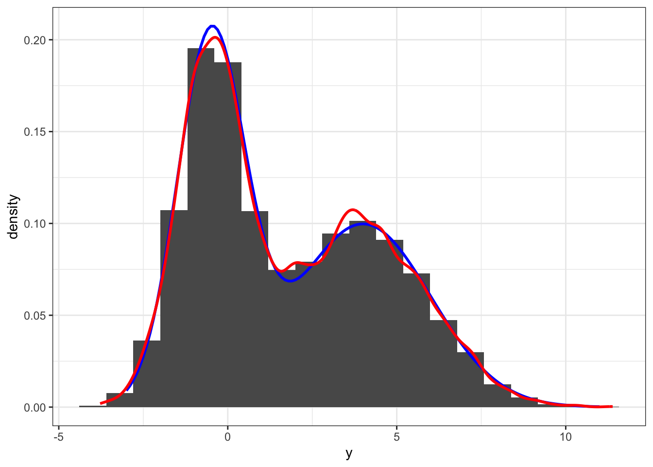
Figure 6.2: Histogram and density estimate (red) of data simulated from a two-component Gaussian mixture distribution. The true mixture distribution has
It is possible to give a mathematically different representation of the marginal distribution of \(Y\) that is sometimes useful. Though it gives the same marginal distribution from the same components, it does provide a different interpretation of what a mixture model is a model of, and it does provide a different way of simulating from a mixture distribution.
If we let \(Y_1 \sim \mathcal{N}(\mu_1, \sigma_1^2)\) and \(Y_2 \sim \mathcal{N}(\mu_2, \sigma_2^2)\) be independent, and independent of \(Z\), we can define
\[\begin{equation} Y = 1(Z = 1) Y_1 + 1(Z = 2) Y_2 = Y_{Z}. \tag{6.2} \end{equation}\]
Clearly, the conditional distribution of \(Y\) given \(Z = k\) is \(f_k\). From (6.2) it follows directly that \[E(Y^N) = P(Z = 1) E(Y_1^N) + P(Z = 2) E(Y_2^N) = p m_1(n) + (1 - p) m_2(n)\] where \(m_k(n)\) denotes the \(N\)th non-central moment of the \(k\)th mixture component. In particular,
\[E(Y) = p \mu_1 + (1 - p) \mu_2.\]
The variance can be found from the second moment as
\[\begin{align} V(Y) & = p(\mu_1^2 + \sigma_1^2) + (1-p)(\mu_2^2 + \sigma_2^2) - (p \mu_1 + (1 - p) \mu_2)^2 \\ & = p\sigma_1^2 + (1 - p) \sigma_2^2 + p(1-p)(\mu_1^2 + \mu_2^2 - 2 \mu_1 \mu_2). \end{align}\]
While it is certainly possible to derive this formula by other means, using (6.2) gives a simple argument based on elementary properties of expectation and independence of \((Y_1, Y_2)\) and \(Z\).
The construction via (6.2) has an interpretation that differs from how a mixture model was defined in the first place. Though \((Y, Z)\) has the correct joint distribution, \(Y\) is by (6.2) the result of \(Z\) selecting one out of two possible observations. The difference can best be illustrated by an example. Suppose that we have a large population consisting of married couples entirely. We can draw a sample of individuals (ignoring the marriage relations completely) from this population and let \(Z\) denote the sex and \(Y\) the height of the individual. Then \(Y\) follows a mixture distribution with two components corresponding to males and females according to the definition. At the risk of being heteronormative, suppose that all couples consist of one male and one female. We could then also draw a sample of married couples, and for each couple flip a coin to decide whether to report the male’s or the female’s height. This corresponds to the construction of \(Y\) by (6.2). We get the same marginal mixture distribution of heights though.
Arguably the heights of individuals in a marriage are not independent, but this is actually immaterial. Any dependence structure between \(Y_1\) and \(Y_2\) is lost in the transformation (6.2), and we can just as well assume them independent for mathematical convenience. We will not be able to tell the difference from observing only \(Y\) (and \(Z\)) anyway.
We illustrate below how (6.2) can be used for alternative implementations of ways to simulate from the mixture model. We compare empirical means and variances to the theoretical values to test if all the implementations actually simulate from the Gaussian mixture model.
## Mean
mu <- p * mu1 + (1 - p) * mu2

## Variance
sigmasq <- p * sigma1^2 + (1 - p) * sigma2^2 +
  p * (1-p)*(mu1^2 + mu2^2 - 2 * mu1 * mu2)

## Simulation using the selection formulation via 'ifelse'
y2 <- ifelse(z, rnorm(n, mu1, sigma1), rnorm(n, mu2, sigma2))

## Yet another way of simulating from a mixture model
## using arithmetic instead of 'ifelse' for the selection
## and with Y_1 and Y_2 actually being dependent
y3 <- rnorm(n)
y3 <- z * (sigma1 * y3 + mu1) + (!z) * (sigma2 * y3 + mu2)

## Returning to the definition again, this last method simulates conditionally
## from the mixture components via transformation of an underlying Gaussian
## variable with mean 0 and variance 1
y4 <- rnorm(n)
y4[z] <- sigma1 * y4[z] + mu1
y4[!z] <- sigma2 * y4[!z] + mu2

## Tests
data.frame(mean = c(mu, mean(y), mean(y2), mean(y3), mean(y4)),
      variance = c(sigmasq, var(y), var(y2), var(y3), var(y4)),
      row.names = c("true", "conditional", "ifelse", "arithmetic",
                    "conditional2" ))
## mean variance
## true 1.750 7.562
## conditional 1.728 7.382
## ifelse 1.713 7.514
## arithmetic 1.708 7.566
## conditional2 1.700 7.464In terms of run time there is not a big difference between three of
the ways of simulating from a mixture model. A benchmark study (not shown) will
reveal that the first and third methods are comparable in terms of run time
and slightly faster than the fourth, while the second using ifelse takes more
than twice as much time as the others. This is
unsurprising as the ifelse method takes (6.2) very literally
and generates twice the number of Gaussian variables actually needed.
The marginal density of \(Y\) is \[f(y) = p \frac{1}{\sqrt{2 \pi \sigma_1^2}} e^{-\frac{(y - \mu_1)^2}{2 \sigma_1^2}} + (1 - p)\frac{1}{\sqrt{2 \pi \sigma_2^2}}e^{-\frac{(y - \mu_2)^2}{2 \sigma_2^2}}\] as given in terms of the parameters \(p\), \(\mu_1, \mu_2\), \(\sigma_1^2\) and \(\sigma_2^2\).
Returning to the canonical parameters we see that they are given as follows: \[\theta_1 = \log \frac{p}{1 - p}, \quad \theta_2 = \frac{\mu_1}{2\sigma_1^2}, \quad \theta_3 = \frac{1}{2\sigma_1^2}, \quad \theta_4 = \frac{\mu_2}{\sigma_2^2}, \quad \theta_5 = \frac{1}{2\sigma_2^2}.\]
The joint density in this parametrization then becomes \[(y,k) \mapsto \left\{ \begin{array}{ll} \exp\left(\theta_1 + \theta_2 y - \theta_3 y^2 - \log (1 + e^{\theta_1}) - \frac{ \theta_2^2}{4\theta_3}+ \frac{1}{2} \log(\theta_3) \right) & \quad \text{if } k = 1 \\ \exp\left(\theta_4 y - \theta_5 y^2 - \log (1 + e^{\theta_1}) - \frac{\theta_4^2}{4\theta_5} + \frac{1}{2}\log(\theta_5) \right) & \quad \text{if } k = 2 \end{array} \right. \] and the marginal density for \(Y\) is
\[\begin{align} f(y \mid \theta) & = \exp\left(\theta_1 + \theta_2 y - \theta_3 y^2 - \log (1 + e^{\theta_1}) - \frac{ \theta_2^2}{4\theta_3}+ \frac{1}{2} \log(\theta_3) \right) \\ & + \exp\left(\theta_4 y - \theta_5 y^2 - \log (1 + e^{\theta_1}) - \frac{\theta_4^2}{4\theta_5} + \frac{1}{2}\log(\theta_5) \right). \end{align}\]
There is no apparent benefit to the canonical parametrization when considering the marginal density. It is, however, of value when we need the logarithm of the joint density as we will for the EM-algorithm.
6.5 Mixed models
A mixed model is a regression model of observations that allows for random variation at two different levels. In this section we will focus on mixed models in an exponential family context. Mixed models can be considered in greater generality but there will then be little shared structure and one has to deal with the models much more on a case-by-case manner.
In a mixed model we have observations \(y_j \in \mathcal{Y}\) and \(z \in \mathcal{Z}\) such that:
- the distribution of \(z\) is an exponential family with canonical parameter \(\theta_0\)
- conditionally on \(z\) the \(y_j\)s are independent with a distribution from an exponential family with sufficient statistics \(t_j( \cdot \mid z)\).
This definition emphasizes how the \(y_j\)s have variation at two levels. There is variation in the underlying \(z\), which is the first level of variation (often called the random effect), and then there is variation among the \(y_j\)s given the \(z\), which is the second level of variation. It is a special case of hierarchical models (Bayesian networks with tree graphs) also known as multilevel models, with the mixed model having only two levels. When we observe data from such a model we typically observe independent replications, \((y_{ij})_{j=1, \ldots, m_i}\) for \(i = 1, \ldots, n\), of the \(y_j\)s only. Note that we allow for a different number, \(m_i\), of \(y_j\)s for each \(i\).
The simplest class of mixed models is obtained by \(t_j = t\) not depending on \(j\), and \[t(y_j \mid z) = \left(\begin{array}{cc} t_1(y_j) \\ t_2(y_j, z) \end{array} \right)\] for some fixed maps \(t_1 : \mathcal{Y} \mapsto \mathbb{R}^{p_1}\) and \(t_2 : \mathcal{Y} \times \mathcal{Z} \mapsto \mathbb{R}^{p_2}\). This is called a random effects model (this is a model where there are no fixed effects in the sense that \(t_j\) does not depend on \(j\), and given the random effect \(z\) the \(y_j\)s are i.i.d.). The canonical parameters associated with such a model are \(\theta_0\) that enters into the distribution of the random effect, \(\theta_1 \in \mathbb{R}^{p_1}\) and \(\theta_2 \in \mathbb{R}^{p_2}\) that enter into the conditional distribution of \(y_j\) given \(z\).
Example 6.5 The special case of a Gaussian, linear random effects model is the model where \(z\) is \(\mathcal{N}(0, 1)\) distributed, \(\mathcal{Y} = \mathbb{R}\) (with base measure proportional to Lebesgue measure) and the sufficient statistic is \[t(y_j \mid z) = \left(\begin{array}{cc} y_j \\ - y_j^2 \\ zy_j \end{array}\right).\] There are no free parameters in the distribution of \(z\).
From Example 6.3 it follows that the conditional variance of \(y\) given \(z\) is \[\sigma^2 = \frac{1}{2\theta_2}\] and the conditional mean of \(y\) given \(z\) is \[\frac{\theta_1 + \theta_3 z}{2 \theta_2} = \sigma^2 \theta_1 + \sigma^2 \theta_3 z.\] Reparametrizing in terms of \(\sigma^2\), \(\beta_0 = \sigma^2 \theta_1\) and \(\nu = \sigma^2 \theta_3\) we see how the conditional distribution of \(y_j\) given \(z\) is \(\mathcal{N}(\beta_0 + \nu z, \sigma^2)\). From this it is clear how the mixed model of \(y_j\) conditionally on \(z\) is a regression model. However, we do not observe \(z\) in practice.
Using the above distributional result we can see that the Gaussian random effects model of observations \(y_{ij}\) can equivalently be stated as
\[Y_{ij} = \beta_0 + \nu Z_i + \varepsilon_{ij}\]
for \(i = 1, \ldots, n\) and \(j = 1, \ldots, m_i\) where \(Z_1, \ldots, Z_N\) are i.i.d. \(\mathcal{N}(0, 1)\)-distributed and independent of \(\varepsilon_{11}, \varepsilon_{12}, \ldots, \varepsilon_{1n_1}, \ldots, \varepsilon_{mn_m}\) that are themselves i.i.d. \(\mathcal{N}(0, \sigma^2)\)-distributed.