2 Density estimation
This chapter is on nonparametric density estimation. A classical nonparametric estimator of a density is the histogram, which provides discontinuous and piecewise constant estimates. The focus in this chapter is on some of the alternatives that provide continuous or even smooth estimates instead.
Kernel methods form an important class of smooth density estimators as
implemented by the R function density(). These estimators are essentially
just locally weighted averages, and their computation is relatively
straightforward in theory. In practice, different choices of how to implement
the computations can, however, have a big effect on the actual runtime,
and the implementation of kernel density estimators will illustrate three points:
- if possible, choose vectorized implementations in R,
- if a small loss in accuracy is acceptable, an approximate solution can be orders of magnitudes faster than a literal implementation,
- the time it takes to numerically evaluate different elementary functions can depend a lot on the function and how you implement the computation.
The first point is emphasized because it results in implementations that are short, expressive and easier to understand just as much as it typically results in computationally more efficient implementations. Note also that not every computation can be vectorized in a beneficial way, and one should never go through hoops to vectorize a computation.
Kernel methods rely on one or more regularization parameters that must be selected to achieve the right balance of adapting to data without adapting too much to the random variation in the data. Choosing the right amount of regularization is just as important as choosing the method to use in the first place. It may, in fact, be more important. We actually do not have a complete implementation of a nonparametric estimator until we have implemented a data driven and automatic way of choosing the amount of regularization. Implementing only the computations for evaluating a kernel estimator, say, and leaving it completely to the user to choose the bandwidth is a job half done. Methods and implementations for choosing the bandwidth are therefore treated in some detail in this chapter.
In the final section a likelihood analysis is carried out. This is done to further clarify why regularized estimators are needed to avoid overfitting to the data, and why there is in general no nonparametric maximum likelihood estimator of a density. Regularization of the likelihood can be achieved by constraining the density estimates to belong to a family of increasingly flexible parametric densities that are fitted to data. This is known as the method of sieves. Another approach is based on basis expansions, but in either case, automatic selection of the amount of regularization is just as important as for kernel methods.
Section 2.2 deals with choosing the bandwidth parameter appropriately. In Section 2.3 we see how likelihood methods can be combined with the use of flexible parametric families of densities. Section 2.4 introduces cross-validation as a general method for choosing tuning parameters, such as the bandwidth parameter or parameters that control the complexity of a parametrized model.
2.1 Kernel methods
Recall the data on \(\phi\)- and \(\psi\)-angles in polypeptide backbone structures, as considered in Section 1.1.1. Figure 2.1 shows histograms of the data. We will in this chapter treat methods for density estimation for univariate data such as data on either the \(\phi\)- or the \(\psi\)-angle.
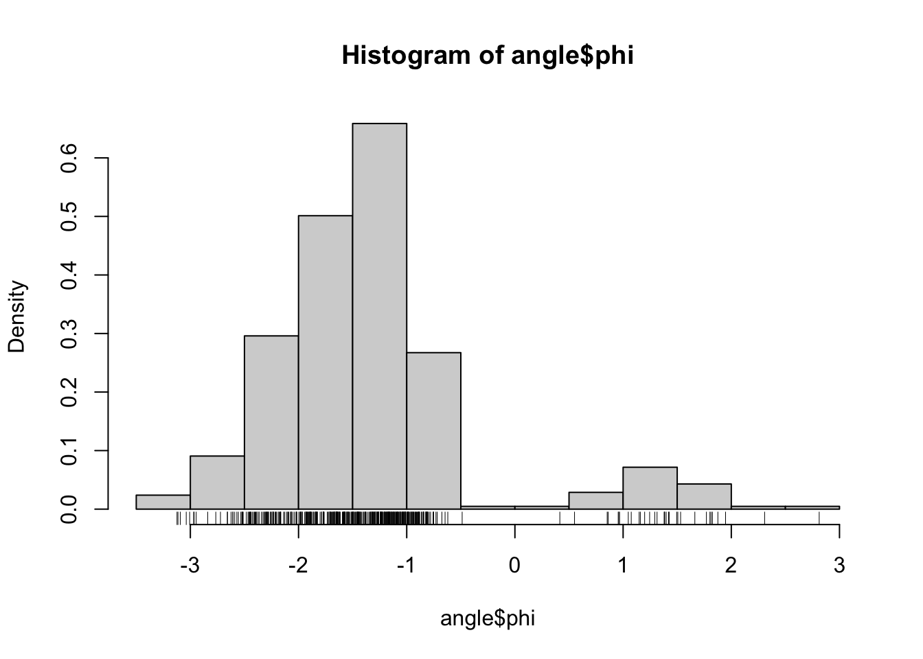
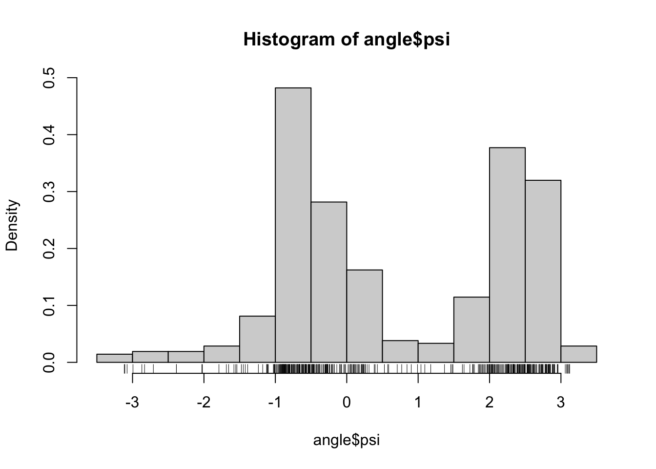
Figure 2.1: Histograms equipped with a rug plot of the distribution of \(\phi\)-angles (left) and \(\psi\)-angles (right) of the peptide planes in the protein human protein 1HMP.
We let \(f_0\) denote the unknown density that we want to estimate. That is, we imagine that the data points \(x_1, \ldots, x_N\) are all observations drawn from the probability measure with density \(f_0\) w.r.t. Lebesgue measure on \(\mathbb{R}\).
In nonparametric density estimating we generally want to estimate the target
density, \(f_0\), without assuming that it belongs to a particular parametrized
family of densities. In this section we develop kernel density
estimation, whose usage via the density() function was illustrated in Section
1.1.
A starting point for nonparametric density estimation is the approximation
\[ \P(X \in (x-h, x+h)) = \int_{x-h}^{x+h} f_0(z) \ dz \approx f_0(x) 2h, \]
which is valid for any continuous density \(f_0\). Inverting this approximation and using the law of large numbers,
\[\begin{align*} f_0(x) & \approx \frac{1}{2h}\P(X \in (x-h, x+h)) \\ & \approx \frac{1}{2hN} \sum_{j=1}^N 1_{(x-h, x+h)}(x_j) \\ & = \underbrace{\frac{1}{2hN} \sum_{j=1}^N 1_{(-h, h)}(x - x_j)}_{\hat{f}_h(x)} \end{align*}\]
for i.i.d. observations \(x_1, \ldots, x_N\) from the distribution with density \(f_0\) w.r.t. Lebesgue measure. The function \(\hat{f}_h\) as defined above is an example of a kernel density estimator using the uniform or rectangular kernel
\[ K(x) = \frac{1}{2} 1_{(-1, 1)}(x) \]
and bandwidth \(h > 0\). The general kernel estimator, is defined as
\[\begin{equation} \hat{f}_h(x) = \frac{1}{hN} \sum_{j=1}^N K\left(\frac{x - x_j}{h}\right) \tag{2.1} \end{equation}\]
for a kernel \(K : \mathbb{R} \to \mathbb{R}\) and a bandwidth parameter \(h > 0\). We often use kernels \(K\) that are non-negative and normalized so that \(\int K(x) \mathrm{d}x = 1\), in which case \(K\) is a pobability density function. A widely used kernel is the Gaussian kernel
\[ K(x) = \frac{1}{\sqrt{2\pi}} e^{-\frac{x^2}{2}}. \]
One direct benefit of considering other kernels than the rectangular is that \(\hat{f}_h\) inherits all smoothness properties from \(K\). Whereas the rectangular kernel is not even continuous, the Gaussian kernel is \(C^{\infty}\) and so is the resulting kernel density estimate. Note also that when \(K\) is a probability density function, \(\hat{f}_h\) is likewise a probability density function. Kernel density estimation is sometimes referred to as the Parzen or Parzen–Rosenblatt window method with reference to their seminal contributions (Rosenblatt 1956; Parzen 1962).
Two natural questions arise when we want to use kernel density estimation in practice. How should we choose the kernel and how should we choose the bandwidth? We discuss below some qualitative effects of these choices on the estimate. In practice the kernel is chosen independently of data based on either computational, statistical or mathematical properties of the kernel—or maybe just based on convenience and availability. The bandwidth is, on the contrary, chosen in a data dependent way, typically to optimize some performance criterion of the estimator. The bandwidth is an example of a tuning parameter, which has to be adjusted appropriately and in a data dependent way for optimal performance of the estimator.
For the rectangular kernel it is fairly easy to understand how the choice of bandwidth qualitatively affects the kernel estimator. We see directly from the definition that \(\hat{f}_h(x)\) is an average over the window \((x-h, x+h)\), and as we move this window over the data points by moving \(x\), \(\hat{f}_h(x)\) will jump up or down depending upon whether a data point is entering or exiting the window. Each jump will be of size \((2hN)^{-1}\) (when all data points are distinct). For large \(h\), the window is large, the jumps are small and \(\hat{f}_h\) will be flat and close to a constant. If \(h\) is small, the window is small and \(\hat{f}_h\) will make larger jumps and be more wiggly. A too large \(h\) will oversmooth the data relative to \(f_0\) by effectively ignoring the data, while a too small \(h\) will undersmooth the data relative to \(f_0\) by allowing individual data points to have large local effects.
The effect of the kernel on the estimator is less obvious. While the bandwidth has a global effect on the density estimate, the kernel’s effect is more local. We noted the most obvious local effect above; that \(\hat{f}_h(x)\) inherits smoothness properties from \(K\). If we consider the rectangular kernel, we may also note that all data points in \((x-h, x+h)\) count equally much. For estimating the density in \(x\) it seems natural that data points close to \(x \pm h\) should count less than points close to \(x\). The rectangular kernel makes a sharp cut at \(x \pm h\); either a data point counts or it does not. Other (smoother) kernels more gradually downweight points further away from \(x\).
Figure 1.5 illustrates how the choice of bandwidth and kernel affects the resulting kernel density estimate. The choice of kernel has relatively minor effects in practice, and we will in this chapter mostly use the Gaussian kernel, but see Exercise 2.1 for an alternative. The choice of bandwidth affects the estimate a lot, and Section 2.2 on bandwidth selection pursues the theory behind automatic and data driven bandwidth selection in more detail. Before going into the details of optimal bandwidth selection we will in the next section treat implementations and computational aspects of kernel density estimation.
2.1.1 Implementation
What does an implementation of a kernel density estimator entail? What
should actually be computed? The definition just specifies how to evaluate
\(\hat{f}_h\) in any given point \(x\), but there is really nothing to compute
until we need to evaluate \(\hat{f}_h.\) There are two different answers to the
question of what to implement. Either we implement \(\hat{f}_h\) as a function
in R, which can compute and return evaluations of \(\hat{f}_h(x)\) for different
\(x\)-s. Or we implement an algorithm
that evaluates and returns the values of the density estimate in a finite number
of points. We will pursue the latter type of implementation, which is
similar to how density() is implemented. The former type of implementation
is discussed in Section 2.3 and Appendix A.2.1.
Our first implementation, kern_dens_loop(), is a fairly low-level
implementation that returns the evaluation of the density estimate in a number
of equidistant points. The function mimics some of the defaults of density()
so that it actually evaluates the estimate in the same points as density().
kern_dens_loop <- function(x, h, n = 512) {
  rg <- range(x)
  # xx is equivalent to grid points in 'density()'
  xx <- seq(rg[1] - 3 * h, rg[2] + 3 * h, length.out = n)
  y <- numeric(n)
  # The computation is done using nested for-loops. The outer loop
  # is over the grid points, and the inner loop is over the data points.
  for (i in seq_along(xx)) {
    for (j in seq_along(x)) {
      y[i] <- y[i] + exp(- (xx[i] - x[j])^2 / (2 * h^2))
    }
  }
  y <- y / (sqrt(2 * pi) * h * length(x))
  list(x = xx, y = y)
}
The function kern_dens_loop() has three formal arguments:
x is the numeric vector of data points, h is the bandwidth
and n is the number of grid points. The default value of n
is 512 matching the default of density().
Note that kern_dens_loop() returns a list containing the grid points (x) where
the density estimate is evaluated as well as the estimated density
evaluations (y).
We test if the implementation works as expected—in this
case by comparing it to density(), which is thus used as a reference
implementation.
f_hat <- kern_dens_loop(angle$psi, 0.2)
f_hat_dens <- density(angle$psi, 0.2)
hist(angle$psi, prob = TRUE, border = NA)
lines(f_hat, lwd = 4, ylab = "Density")
lines(f_hat_dens, col = "red", lwd = 2)
plot(f_hat$x, f_hat$y - f_hat_dens$y,
  type = "l",
  lwd = 2,
  xlab = "psi",
  ylab = "Difference"
)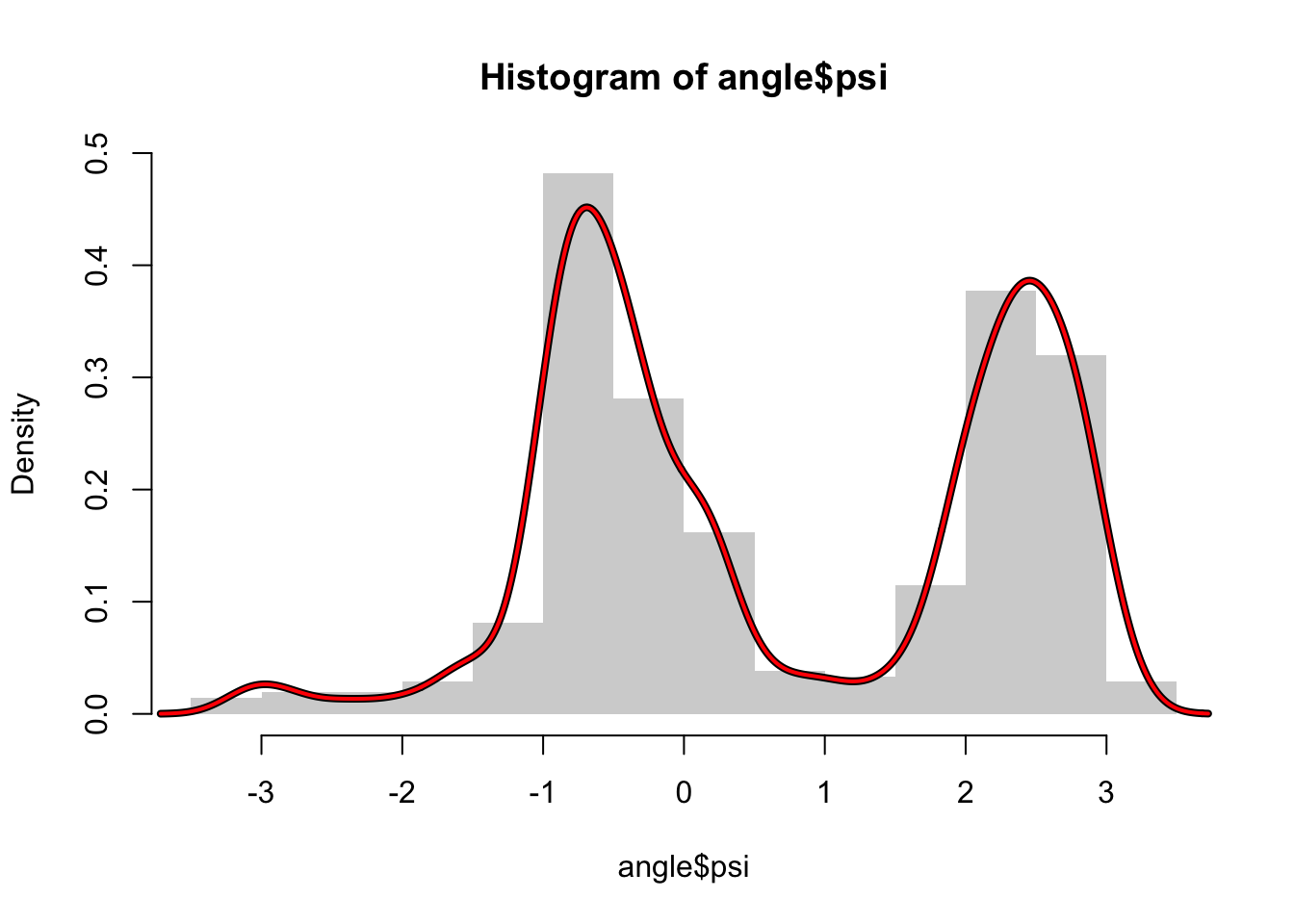

Figure 2.2: Kernel density estimates with the Gaussian kernel (left) using R’s implementation (black) and our implementation (red) together with differences of the estimates (right).
Figure 2.2 suggests that the estimates computed by our
implementation and by density() are the same when we just visually compare the
plotted densities. However, if we look at the differences instead,
we see that the differences can be as large as \(4 \times 10^{-4}\) in absolute value. This is
way above what we should expect from rounding errors alone when using
double precision arithmetic. Thus the two implementations only compute
approximately the same. The reason for these differences is that
density() actually relies on certain approximations for runtime
efficiency.
In R we can often beneficially implement computations in a vectorized way
instead of using an explicit loop. It is fairly easy to change the implementation
to be more vectorized by computing each evaluation in one single line using
the sum() function and the fact that exp() and squaring are vectorized.
kern_dens_vec <- function(x, h, n = 512) {
  rg <- range(x)
  xx <- seq(rg[1] - 3 * h, rg[2] + 3 * h, length.out = n)
  y <- numeric(n)
  # The inner loop from 'kern_dens_loop()' has been vectorized, and
  # only the outer loop over the grid points remains.
  const <- (sqrt(2 * pi) * h * length(x))
  for (i in seq_along(xx)) {
      y[i] <- sum(exp(-(xx[i] - x)^2 / (2 * h^2))) / const
  }
  list(x = xx, y = y)
}
We test this new implementation by comparing it to our previous implementation.
range(kern_dens_loop(angle$psi, 0.2)$y - kern_dens_vec(angle$psi, 0.2)$y)## [1] 0 0The magnitude of the differences are of order at most \(10^{-16}\), which is what
can be expected due to rounding errors. Thus we conclude that up to rounding
errors, kern_dens_loop() and kern_dens_vec() return the same on this dataset. This is,
of course, not a comprehensive test, but it is an example of one among a
number of tests that should be considered.
There are several ways to get completely rid of the explicit loops and write
an entirely vectorized implementation in R. One of the solutions will use the
vapply() function, which belongs to the family of *apply() functions
in base R that apply a function to each element in a vector or a list. In the
parlance of functional programming the *apply() functions are variations
of the functional, or higher-order-function, known as map.
kern_dens_apply <- function(x, h, n = 512) {
  rg <- range(x)
  xx <- seq(rg[1] - 3 * h, rg[2] + 3 * h, length.out = n)
  const <- sqrt(2 * pi) * h * length(x)
  kern <- function(z) sum(exp(-(z - x)^2 / (2 * h^2))) / const
  y <- vapply(xx, kern, FUN.VALUE = double(1))
  list(x = xx, y = y)
}
The vapply() call applies the function kern(),
defined in the line before, to every element in the vector xx. The
FUN.VALUE = double(1) specifies that the return value of kern()
is a double and that vapply() should return a vector of doubles.
An alternative to vapply() is lapply(), which always returns a list,
or sapply(), which is a simple wrapper around lapply() that attempts
to “simplify” the result from a list to an array. For programming,
it is safest to use vapply() or lapply() since these functions always
return an object of the same type, while sapply() can return a list as
well as a vector or an array depending on the circumstances. Going beyond
base R, the purrr package offers a different implementation of maps and
functionals.
An alternative, and also completely vectorized, solution is based on
the functions outer() and rowMeans().
kern_dens_outer <- function(x, h, n = 512) {
  rg <- range(x)
  xx <- seq(rg[1] - 3 * h, rg[2] + 3 * h, length.out = n)
  y <- outer(xx, x, function(zz, z) exp(- (zz - z)^2 / (2 * h^2)))
  y <- rowMeans(y) / (sqrt(2 * pi) * h)
  list(x = xx, y = y)
}
The outer() function evaluates the kernel in all combinations of the grid and
data points and returns a matrix of dimensions \(N \times N\). The function
rowMeans() computes the means of each row and returns a vector of length \(N\).
Note how the third argument to outer() is an anonymous function. That is, it
is a function that does not get a name and exists only during the evaluation of
the outer() call. It is immaterial for the result and efficiency of the
computation whether a function gets a name, like kern() in the implementation
of kern_dens_apply(), or if it is anonymous as in the implementation of
kern_dens_outer(). But it does affect the readability of the code. It is fine
to use simple anonymous functions, but more complicated functions spanning multiple
lines of code should preferably be separated out and given a name.
We should, of course, remember to test the two last implementations, e.g.,
by comparing with kern_dens_loop().
range(kern_dens_loop(angle$psi, 0.2)$y - kern_dens_apply(angle$psi, 0.2)$y)## [1] 0 0
range(kern_dens_loop(angle$psi, 0.2)$y - kern_dens_outer(angle$psi, 0.2)$y)## [1] -5.551e-17 5.551e-17The natural question is how to choose between the different implementations?
Besides being correct it is important that the code is easy to read
and understand. Which of the four implementations above that is best in
this respect may depend a lot on the background of the reader.
All four implementations are arguably quite readable, but
kern_dens_loop() with the double loop might appeal a bit more to people
with a background in imperative programming, while kern_dens_apply() might
appeal more to people with a preference for functional programming.
This functional and vectorized solution is also
a bit closer to the mathematical notation with,
e.g., the sum sign \(\Sigma\) being mapped directly to the sum() function
instead of the incremental addition in the for-loop. For
these specific implementations the differences are mostly
aesthetic nuances and preferences may be more subjective than substantial.
To make a qualified choice between the implementations we should investigate if they differ in terms of runtime and memory consumption.
2.1.2 Benchmarking
Benchmarking is about measuring and comparing performance. For software this often means measuring runtime and memory usage, though there are clearly many other aspects of software that should be benchmarked in general. This includes user experience, energy consumption and implementation and maintenance time. In this section we focus on benchmarking runtime and memory usage.
Base R provides a simple way of measuring runtime via the function system.time().
Throughout this book we will use the tools from the bench package to benchmark
code, see also Appendix A.3. It includes the bench_time()
function as an alternative to system.time() for measuring
the time it takes to evaluate a single expression.
bench::bench_time(kern_dens_loop(angle$psi, 0.2))
bench::bench_time(kern_dens_vec(angle$psi, 0.2))
bench::bench_time(kern_dens_apply(angle$psi, 0.2))
bench::bench_time(kern_dens_outer(angle$psi, 0.2))
## kern_dens_loop:
## process real
## 17.7ms 17.4ms
## kern_dens_vec:
## process real
## 1.24ms 1.23ms
## kern_dens_apply:
## process real
## 1.39ms 1.36ms
## kern_dens_outer:
## process real
## 1.38ms 1.36msThe bench package does high precision benchmarking and offers a range of
convenient tools, including good default formatting options so that all timings
are printed in a human readable way with correct units. The
bench_time() function prints out two measurements.
The “real” time is the total runtime, also known as the “wallclock time”,
while the “process” time is the time that the CPU actually spent on the
expression evaluation. Curiously, for fast evaluations as above, the
wallclock time can be smaller than the process time if the two are not
measured with the same precision (and this is the case on macOS).
From this simple benchmark, kern_dens_loop() is clearly substantially slower
than the three other implementations. For more systematic benchmarking of
runtime we use the mark() function from the bench package, which evaluates
expressions repeatedly to give a more complete picture of the distribution
of runtime and memory usage, see also Appendix A.3.
kern_bench <- bench::mark(
  loop = kern_dens_loop(angle$psi, 0.2),
  vec = kern_dens_vec(angle$psi, 0.2),
  apply = kern_dens_apply(angle$psi, 0.2),
  outer = kern_dens_outer(angle$psi, 0.2)
)
Note that mark() by default checks that the results from all benchmarked
expressions are (nearly) equal by all.equal(), thus the above benchmarking
also implicitly tests consistency of the implementations. The result stored in
kern_bench is a tabular data structure with one row for each expression
benchmarked and a good default print method for showing summary statistics
from the benchmark.
## # A tibble: 4 × 6
##   expression      min   median `itr/sec` mem_alloc `gc/sec`
##   <bch:expr> <bch:tm> <bch:tm>     <dbl> <bch:byt>    <dbl>
## 1 loop        16.94ms  17.43ms      57.3   21.53KB      0
## 2 vec          1.09ms   1.22ms     809.     1.68MB     37.6
## 3 apply        1.24ms   1.41ms     709.     1.68MB     35.3
## 4 outer        1.08ms   1.36ms     732.     4.93MB    157.
The median runtimes are similar to the measurements done using
bench_time(). The implementation of the kernel density estimator
using a double loop takes 15–16 ms, while
the three vectorized implementations take about 1.3 ms and are thus more than a
factor 10 faster. The memory allocation is, however, larger for all vectorized
implementations and largest for the implementation using outer().
To visualize the complete banchmark data behind the summary statistics we can use the plot method for benchmark data. It is based on ggplot2 and thus easy to modify, and we change a few defaults here for a better presentation of the results.
library(bench)
plot(kern_bench) +
    scale_x_discrete(limits = c("outer", "apply", "vec", "loop")) +
    bench::scale_y_bench_time(breaks = c(1, 3, 10, 30, 100) * 10^{-3})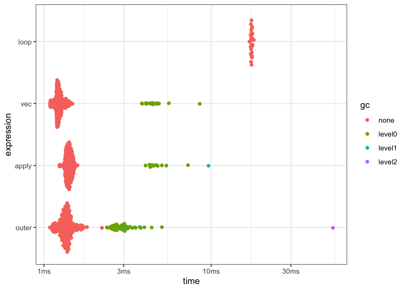
The more refined benchmark study using mark() does not change our initial impression from
using bench_time() substantially. The function kern_dens_loop() is notably
slower than the three vectorized implementations, but we are now able to
more clearly see the minor differences among them. It appears that
kern_dens_apply() and kern_dens_outer() have somewhat similar
runtime distributions and that kern_dens_vec() is marginally faster than
both of these. Other minor differences in these empirical runtime distributions
change if the experiment is repeated.
Garbage collection.
2.1.3 Runtime complexity
In many cases when we benchmark runtime it is of interest
to investigate how runtime depends on various parameters. This is so
for kernel density estimation, where we want to understand how changes in
the number of data points, \(N\), and the number of grid points, \(n\), affect
runtime. The function press() from the bench package can be used to
run benchmarks across a grid of parameters, and it will “press” the
results together in a tabular data structure.
x <- rnorm(2^11)
kern_benchmarks <- bench::press(
  N = 2^(5:11),
  n = 2^c(5, 7, 9, 11),
  {
    bench::mark(
      loop = kern_dens_loop(x[1:N], h = 0.2, n = n),
      vec = kern_dens_vec(x[1:N], h = 0.2, n = n),
      apply = kern_dens_apply(x[1:N], h = 0.2, n = n),
      outer = kern_dens_outer(x[1:N], h = 0.2, n = n)
    )
  }
)
## Warning: Some expressions had a GC in every iteration; so filtering is
## disabled.
head(kern_benchmarks)## # A tibble: 6 × 8
## expression N n min median `itr/sec` mem_alloc `gc/sec`
## <bch:expr> <dbl> <dbl> <bch:tm> <bch:tm> <dbl> <bch:byt> <dbl>
## 1 loop 32 32 84µs 92µs 10853. 1.77KB 4.06
## 2 vec 32 32 18.8µs 21.7µs 42185. 10.97KB 16.9
## 3 apply 32 32 28.7µs 32.4µs 30200. 10.97KB 21.2
## 4 outer 32 32 15.7µs 17.7µs 54437. 25.61KB 27.2
## 5 loop 64 32 159.7µs 174.5µs 5704. 2.56KB 2.02
## 6 vec 64 32 23.6µs 26.8µs 36699. 19.77KB 14.7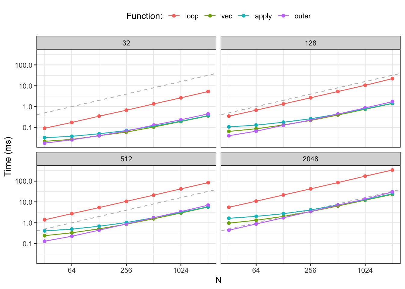
Figure 2.3: Median runtime for the four different implementations of kernel density estimation. The dashed gray line is a reference line with slope 1.
Figure 2.3 shows median runtimes for an experiment with 28
combinations of parameters for each of the four different implementations
yielding a total of 112 different R expressions being benchmarked. The results
confirm that kern_dens_loop() is substantially slower than the vectorized
implementations for all combinations of \(N\) and \(n\). However, Figure
2.3 also reveals a new pattern; kern_dens_outer()
appears to scale with \(N\) in a slightly different way than the two other
vectorized implementations for small \(N\). It is comparable to or even a bit
faster than kern_dens_vec() and kern_dens_apply() for very small datasets,
while it becomes slower for the larger datasets.
Runtime for many algorithms have to a good approximation a dominating power law behavior as a function of typical size parameters, that is, the runtime will scale approximately like \(N \mapsto C N^a\) for constants \(C\) and \(a\) and with \(N\) denoting a size parameter (number of data points, say). Therefore it is beneficial to plot runtime using log-log scales and to design benchmark studies with size parameters being equidistant on a log-scale. With approximate power law scaling, the log runtime behaves like
\[ \log(C) + a \log(N), \]
that is, on a log-log scale we see approximate straight lines. The slope reveals the exponent \(a\), and two different algorithms for solving the same problem might have different exponents and thus different slopes on the log-log-scale. Two different implementations of the same algorithm should have approximately the same slope but may differ in the constant \(C\) depending upon how efficient the particular implementation is in the particular programming language used. Differences in \(C\) correspond to vertical translations on the log-log scale.
In practice, we will see some deviations from straight lines on the log-log plot for a number of reasons. Writing the runtime as \(C N^a + R(N)\), the residual term \(R(N)\) will often be noticeable or even dominating and positive for small \(N\). It is only for large enough \(N\) that the power law term, \(C N^a\), will dominate. In addition, runtime can be affected by hardware constraints such as cache and memory sizes, which can cause abrupt jumps in runtime.
2.2 Bandwidth selection
We show in this section that optimal bandwidth selection can be seen as a bias-variance tradeoff. To quantify how good a specific estimate \(\hat{f}_h\) is, we introduce the integrated squared error,
\[ \mathrm{ISE}(\hat{f}_h) = \int (\hat{f}_h(x) - f_0(x))^2 \ \mathrm{d}x = \|\hat{f}_h - f_0\|_2^2. \]
The quality of the estimation procedure producing \(\hat{f}_h\) from data can then be quantified by taking the mean ISE,
\[ \mathrm{MISE}(h) = \E(\mathrm{ISE}(\hat{f}_h)), \]
where the expectation in an integral over the data distribution. Using Tonelli’s theorem we may interchange the expectation and the integration over \(x\) to get
\[ \mathrm{MISE}(h) = \int \mathrm{MSE}_h(x) \ \mathrm{d}x \]
where
\[ \mathrm{MSE}_h(x) = \E(\hat{f}_h(x) - f_0(x))^2 \]
is the mean squared error in \(x\). Introducing the mean of the kernel density estimator \(\hat{f}_h\) as
\[\begin{equation} \label{eq:dens-mean} f_h(x) = \E(\hat{f}_h(x)), \end{equation}\]
we can then also write
\[\begin{align*} \mathrm{MSE}_h(x) & = \E(\hat{f}_h(x) - f_h(x))^2 + (f_h(x) - f_0(x))^2 \\ & = \V(\hat{f}_h(x)) + \mathrm{bias}(\hat{f}_h(x))^2. \end{align*}\]
We thus have
\[ \mathrm{MISE}(h) = \int \V(\hat{f}_h(x)) \ \mathrm{d}x + \int \mathrm{bias}(\hat{f}_h(x))^2 \ \mathrm{d}x. \]
Choosing \(h\) by minimizing \(\mathrm{MISE}(h)\) can thus be seen as finding a suitable tradeoff between the integrated variance and integrated squared bias. Before proceeding with the general theory, we focus again on the rectangular kernel where some computations are simpler.
2.2.1 Revisiting the rectangular kernel
For the rectangular kernel, and with \(p(x, h) = \P(X \in (x-h, x+h))\), we find that
\[\begin{align} f_h(x) & = p(x, h) / (2h) \tag{2.2} \\ \V(\hat{f}_h(x)) & = \frac{p(x, h) (1 - p(x, h))}{4h^2 N} \approx f_h(x) \frac{1}{2hN}, \tag{2.3} \end{align}\]
with the approximation valid for \(h\) small. We see from these computations that for \(\hat{f}_h(x)\) to be approximately unbiased for any \(x\) we need \(h\) to be small—ideally letting \(h \to 0\) since then \(f_h(x) \to f_0(x)\). However, this will make the variance blow up, and to minimize variance we should instead choose \(h\) as large as possible. An appropriate choice of \(h\) strikes a balance between the bias and the variance as a function of \(h\) by minimizing the mean squared error of \(\hat{f}_h(x)\).
To carry out a more rigorous analysis we assume that \(f_0\) is sufficiently differentiable. For the derivation it may be helpful to think of \(N\) as large and \(h\) as small. Indeed, we will eventually choose \(h = h_N\) as a function of \(N\) such that as \(N \to \infty\) we have \(h_N \to 0\). We also note the \(f_h(x)\) is a density, thus \(\int f_h(x) \mathrm{d}x = 1\).
We use a Taylor expansion of the distribution function \(F_0\) to get that
\[\begin{align*} f_h(x) & = \frac{1}{2h}\left(F_0(x + h) - F_0(x - h)\right) \\ & = \frac{1}{2h}\left(2h f_0(x) + \frac{h^3}{3} f_0''(x) + R_0(x,h) \right) \\ & = f_0(x) + \frac{h^2}{6} f_0''(x) + R_1(x,h) \end{align*}\]
where \(R_1(x, h) = o(h^2)\). One should note how the quadratic terms in \(h\) in the Taylor expansion canceled. This gives the following formula for the squared bias of \(\hat{f}_h\).
\[\begin{align*} \mathrm{bias}(\hat{f}_h(x))^2 & = (f_h(x) - f_0(x))^2 \\ & = \left(\frac{h^2}{6} f_0''(x) + R_1(x,h) \right)^2 \\ & = \frac{h^4}{36} f_0''(x)^2 + R(x,h) \end{align*}\]
where \(R(x,h) = o(h^4)\). For the variance we see from (2.3) that
\[ \V(\hat{f}_h(x)) = f_h(x)\frac{1}{2Nh} - f_h(x)^2 \frac{1}{N}. \]
Integrating the sum of the bias and the variance over \(x\) gives the integrated mean squared error
\[\begin{align*} \mathrm{MISE}(h) & = \int \mathrm{bias}(\hat{f}_h(x))^2 + \V(\hat{f}_h(x)) \mathrm{d}x \\ & = \frac{h^4}{36} \|f_0''\|^2_2 + \frac{1}{2hN} + \int R(x,h) \mathrm{d} x - \frac{1}{N} \int f_h(x)^2 \mathrm{d} x. \end{align*}\]
If \(f_h(x) \leq C\) (which happens if \(f_0\) is bounded),
\[ \int f_h(x)^2 \mathrm{d} x \leq C \int f_h(x) \mathrm{d} x = C, \]
and the last term is \(o((Nh)^{-1})\). The second last term is \(o(h^4)\) if we can interchange the limit and integration order. It is conceivable that we can do so under suitable assumptions on \(f_0\), but we will not pursue those at this place. The sum of the two remaining and asymptotically dominating terms in the formula for MISE is
\[ \mathrm{AMISE}(h) = \frac{h^4}{36} \|f_0''\|^2_2 + \frac{1}{2N h}, \]
which is known as the asymptotic mean integrated squared error. Clearly, for this to be a useful formula, we must assume \(\|f_0''\|_2^2 < \infty\). In this case the formula for AMISE can be used to find the asymptotic optimal tradeoff between integrated bias and variance. Differentiating w.r.t. \(h\) we find that
\[ \mathrm{AMISE}'(h) = \frac{h^3}{9} \|f_0''\|^2_2 - \frac{1}{2N h^2}, \]
and solving for \(\mathrm{AMISE}'(h) = 0\) yields
\[ h_N = \left(\frac{9}{2 \|f_0''\|_2^2}\right)^{1/5} N^{-1/5}. \]
When AMISE is regarded as a function of \(h\) we observe that it tends to \(\infty\) for \(h \to 0\) as well as for \(h \to \infty\), thus the unique stationary point \(h_N\) is a unique global minimizer. Choosing the bandwidth to be \(h_N\) will therefore minimize the asympototic mean integrated squared error, and it is in this sense an optimal choice of bandwidth.
We see how “wiggliness” of \(f_0\) enters into the formula for the optimal bandwidth \(h_N\) via \(\|f_0''\|_2\). This norm of the second derivative is precisely a quantification of how much \(f_0\) oscillates. A large value, indicating a wiggly \(f_0\), will drive the optimal bandwidth down whereas a small value will drive the optimal bandwidth up.
We should also observe that if we plug the optimal bandwidth into the formula for AMISE, we get
\[\begin{align*} \mathrm{AMISE}(h_N) & = \frac{h_N^4}{36} \|f_0''\|^2_2 + \frac{1}{2N h_N } \\ & = C N^{-4/5}, \end{align*}\]
which indicates that in terms of integrated mean squared error the rate at which we can nonparametrically estimate \(f_0\) is \(n^{-4/5}\). This should be contrasted to the common parametric rate of \(n^{-1}\) for mean squared error.
From a practical viewpoint there is one major problem with the optimal bandwidth \(h_N\); it depends via \(\|f_0''\|^2_2\) upon the unknown \(f_0\) that we are trying to estimate. We therefore refer to \(h_N\) as an oracle bandwidth—it is the bandwidth that an oracle that knows \(f_0\) would tell us to use. In practice, we will have to come up with an estimate of \(\|f_0''\|^2_2\) and plug that estimate into the formula for \(h_N\). We pursue a couple of different options for doing so for general kernel density estimators below together with methods that do not rely on the AMISE formula.
2.2.2 The oracle bandwidth and its estimation
We can generalize the computations for the rectangular kernel in the section above to any kernel, subject to some regularity conditions. To this end we define the asymptotic mean integrated squared error as
\[ \mathrm{AMISE}(h) = \frac{\|K\|_2^2}{nh} + \frac{h^4 \sigma^4_K \|f_0''\|_2^2}{4} \]
with
\[ \|g\|_2^2 = \int g(x)^2 \ \mathrm{d}x \quad (\mathrm{squared } \ L_2\mathrm{-norm}). \]
and \(\sigma_K^2 = \int x^2 K(x) \ \mathrm{d}x\).
For \(\mathrm{AMISE}(h)\) to be well defined and finite we need the density \(f_0\) to be twice differentiable, we need both \(f_0''\) and the kernel, \(K\), to be square integrable, and we need \(\sigma_K^2\) to be finite. When the kernel is a density, these conditions turn out to also be sufficient to express the asymptotic behavior of \(\mathrm{MISE}(h)\) in terms of \(\mathrm{AMISE}(h)\).
Theorem 2.1 Suppose the kernel \(K\) is a square integrable density for a probability distribution on \(\mathbb{R}\). If
\[ \sigma_K^2 = \int x^2 K(x) \ \mathrm{d}x \in (0, \infty), \]
and if \(f_0\) is twice differentiable with if \(f_0''\) square integrable,
\[ \mathrm{MISE}(h) = \mathrm{AMISE}(h) + o((Nh)^{-1} + h^4). \]
The proof of Theorem 2.1 can be based on the same kind of Taylor expansion argument as in Section 2.2.1. See Proposition A.1 in Tsybakov (2009) for a rigorous proof, where remainder terms are handled carefully.
By minimizing \(\mathrm{AMISE}(h)\) we derive the asymptotically optimal oracle bandwidth
\[\begin{equation} \tag{2.4} h_N = \left( \frac{\|K\|_2^2}{ \|f_0''\|^2_2 \sigma_K^4} \right)^{1/5} n^{-1/5}. \end{equation}\]
If we plug this formula into the formula for AMISE we arrive at the asymptotic error rate \(\mathrm{AMISE}(h_N) = C N^{-4/5}\) with a constant \(C\) depending on \(f_0''\) and the kernel.
It is noteworthy that the asymptotic analysis can be carried out even if \(K\) is allowed to take negative values. Then \(K\) is not a density and the resulting estimate may not be a valid density as it is. Tsybakov (2009) demonstrates how to improve on the rate \(N^{-4/5}\) by allowing for kernels whose moments of order two or above vanish. Necessarily, such kernels must take negative values and cannot be densities.
We observe that for the rectangular kernel,
\[ \sigma_K^4 = \left(\frac{1}{2} \int_{-1}^1 z^2 \ \mathrm{d} z\right)^2 = \frac{1}{9} \]
and
\[ \|K\|_2^2 = \frac{1}{2^2} \int_{-1}^1 \ \mathrm{d} z = \frac{1}{2}. \]
Plugging these numbers into (2.4) we find the oracle bandwidth for the rectangular kernel as derived in Section 2.2.1. For the Gaussian kernel we find that \(\sigma_K^4 = 1\), while
\[ \|K\|_2^2 = \frac{1}{2 \pi} \int e^{-x^2} \ \mathrm{d} x = \frac{1}{2 \sqrt{\pi}}. \]
The major practical problem with the oracle bandwidth is that it depends on \(\|f_0''\|^2_2\). Thus to compute the asymptotically optimal bandwidth we have to know the second derivative of \(f_0\) that we are trying to estimate in the first place. To resolve the circularity we will make a first guess of what \(f_0\) is and plug that guess into the formula for the oracle bandwidth.
Our first guess is that \(f_0\) is Gaussian with mean 0 and variance \(\sigma^2\). Then
\[\begin{align*} \|f_0''\|^2_2 & = \frac{1}{2 \pi \sigma^2} \int \left(\frac{x^2}{\sigma^4} - \frac{1}{\sigma^2}\right)^2 e^{-x^2/\sigma^2} \ \mathrm{d}x \\ & = \frac{1}{2 \sigma^9 \sqrt{\pi}} \frac{1}{\sqrt{\pi \sigma^2}} \int (x^4 - 2 \sigma^2 x^2 + \sigma^4) e^{-x^2/\sigma^2} \ \mathrm{d}x \\ & = \frac{1}{2 \sigma^9 \sqrt{\pi}} (\frac{3}{4} \sigma^4 - \sigma^4 + \sigma^4) \\ & = \frac{3}{8 \sigma^5 \sqrt{\pi}}. \end{align*}\]
Plugging this expression for the squared 2-norm of the second derivative of the density into the formula for the oracle bandwidth gives
\[\begin{equation} \tag{2.5} h_N = \left( \frac{8 \sqrt{\pi} \|K\|_2^2}{3 \sigma_K^4} \right)^{1/5} \sigma n^{-1/5}, \end{equation}\]
with \(\sigma\) the only quantity depending on the unknown density \(f_0\). We can now simply estimate \(\sigma\), using, e.g., the empirical standard deviation \(\hat{\sigma}\), and plug this estimate into the formula above to get an estimate of the oracle bandwidth.
It is well known that the empirical standard deviation is sensitive to outliers, and if \(\sigma\) is overestimated for that reason, the bandwidth will be too large and the resulting estimate will be oversmoothed. To get more robust bandwidth selection, Silverman (1986) suggested using the interquartile range to estimate \(\sigma\). In fact, he suggested estimating \(\sigma\) by
\[ \tilde{\sigma} = \min\{\hat{\sigma}, \mathrm{IQR} / 1.34\}. \]
In this estimator, IQR denotes the empirical interquartile range, and \(1.34\) is approximately the interquartile range, \(\Phi^{-1}(0.75) - \Phi^{-1}(0.25)\), of the standard Gaussian distribution. Curiously, the interquartile range for the standard Gaussian distribution is \(1.35\) to two decimals accuracy, but the use of \(1.34\) in the estimator \(\tilde{\sigma}\) has prevailed. Silverman, moreover, suggested to reduce the kernel-dependent constant in the formula (2.5) for \(h_N\) to further reduce oversmoothing.
If we specialize to the Gaussian kernel, formula (2.5) simplifies to
\[ \hat{h}_N = \left(\frac{4}{3}\right)^{1/5} \tilde{\sigma} n^{-1/5}, \]
with \(\tilde{\sigma}\) plugged in as a robust estimate of \(\sigma\). Silverman (1986) made the ad hoc suggestion to reduce the factor \((4/3)^{1/5} \approx 1.06\) to \(0.9\). This results in the bandwidth estimate
\[ \hat{h}_N = 0.9 \tilde{\sigma} n^{-1/5}, \]
which has become known as Silverman’s rule of thumb.
Silverman’s rule of thumb is the default bandwidth estimator for density()
as implemented by the function bw.nrd0(). The bw.nrd() function implements
bandwidth selection using the factor \(1.06\) instead of \(0.9\). Though the theoretical
derivations behind these implementations assume that \(f_0\)
is Gaussian, either will give reasonable bandwidth selection for a range of
unimodal distributions. If \(f_0\) is multimodal, Silverman’s
rule of thumb is known to oversmooth the density estimate.
Instead of computing \(\|f_0''\|^2_2\) assuming that the distribution is Gaussian, we can compute the norm for a pilot estimate, \(\tilde{f}\), and plug the result into the formula for \(h_N\). If the pilot estimate is a kernel estimate with kernel \(H\) and bandwidth \(r\) we get
\[ \|\tilde{f}''\|^2_2 = \frac{1}{n^2r^6} \sum_{i = 1}^N \sum_{j=1}^N \int H''\left( \frac{x - x_i}{r} \right) H''\left( \frac{x - x_j}{r} \right) \mathrm{d} x. \]
The problem is, of course, that now we have to choose the pilot bandwidth \(r\). But doing so using a simple method like Silverman’s rule of thumb at this stage is typically not too bad an idea. Thus we arrive at the following plug-in procedure using the Gaussian kernel for the pilot estimate:
- Compute an estimate, \(\hat{r}\), of the pilot bandwidth using Silverman’s rule of thumb.
- Compute \(\|\tilde{f}''\|^2_2\) using the Gaussian kernel as pilot kernel \(H\) and using the estimated pilot bandwidth \(\hat{r}\).
- Plug \(\|\tilde{f}''\|^2_2\) into the oracle bandwidth formula (2.4) to compute \(\hat{h}_N\) for the kernel \(K\).
Note that to use a pilot kernel different from the Gaussian we have to adjust the constant 0.9 (or 1.06) in Silverman’s rule of thumb accordingly by computing \(\|H\|_2^2\) and \(\sigma_H^4\) and using (2.5).
Sheather and Jones (1991) took these plug-in ideas a step further and analyzed in detail
how to choose the pilot bandwidth in a good and data adaptive way. The resulting
method is somewhat complicated but implementable. We skip the details but simply
observe that their method is implemented in R in the function bw.SJ(), and
it can be selected when using density() by setting the argument bw = "SJ".
This plug-in method is regarded as a solid default that performs well for
many different data generating densities \(f_0\).
f_hat_nrd <- kern_dens_vec(angle$psi, bw.nrd(angle$psi))
f_hat_nrd0 <- kern_dens_vec(angle$psi, bw.nrd0(angle$psi))
f_hat_SJ <- kern_dens_vec(angle$psi, bw.SJ(angle$psi))
hist(angle$psi, prob = TRUE, border = NA)
lines(f_hat_nrd, col = "blue", lwd = 2)
lines(f_hat_nrd0, col = "red", lwd = 2)
lines(f_hat_SJ, col = "purple", lwd = 2)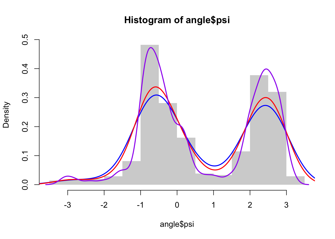
2.3 Parametric models
As an alternative to the ad hoc nonparametric kernel density estimator, we could also approximate the density \(f_0\) by a density from a parametrized statistical model \((f_{\theta})_{\theta \in \Theta}\), where \(f_{\theta}\) is a density w.r.t. Lebesgue measure on \(\mathbb{R}\) for each parameter \(\theta \in \Theta\). If \(\hat{\theta}\) is an estimate of the parameter, \(f_{\hat{\theta}}\) is an estimate of the unknown density \(f_0\). For a parametric family we can always try to use the maximum-likelihood estimator
\[ \hat{\theta} = \argmax_{\theta} \sum_{j=1}^N \log f_{\theta}(x_j) \]
as an estimate of \(\theta\). If the parametrized family of distributions is the family of Gaussian distributions, we can estimate the mean and variance parameters by the empirical mean and variance for the data and plug those numbers into the density for the Gaussian distribution. In this way obtain a Gaussian density estimate of \(f_0\).
psi_mean <- mean(angle$psi)
psi_sd <- sd(angle$psi)
hist(angle$psi, prob = TRUE)
rug(angle$psi)
curve(dnorm(x, psi_mean, psi_sd), add = TRUE, col = "red")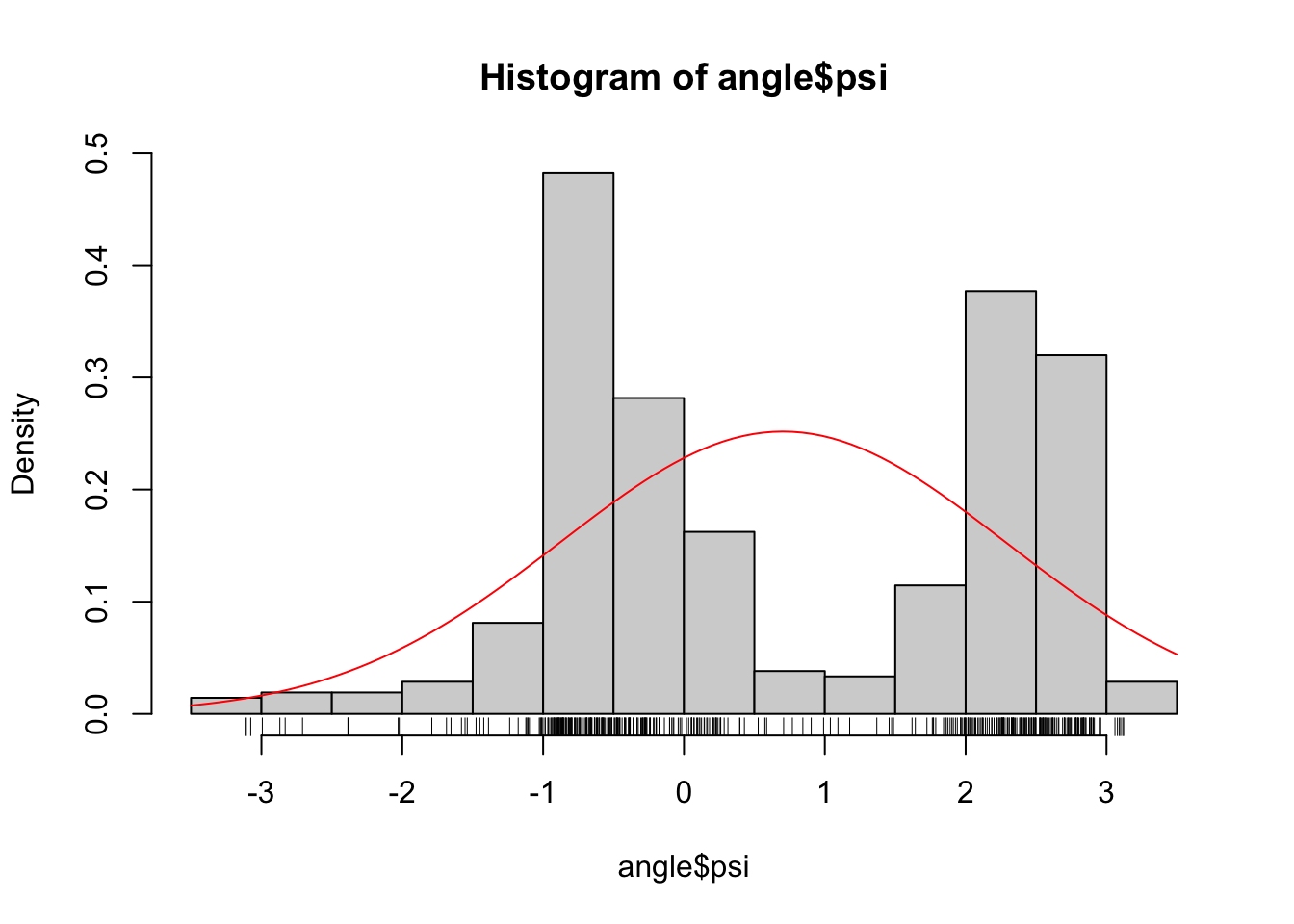
Figure 2.5: Gaussian density (red) fitted to the \(\psi\)-angles.
As Figure 2.5 shows, if we fit a Gaussian distribution to the \(\psi\)-angle data we get a density estimate that clearly does not match the histogram. The Gaussian density matches the data on the first and second moments, but the histogram shows a bimodality that the Gaussian density can never match. Thus we need a more flexible model than the family of Gaussian distributions. Could we go all-in and simply maximize the likelihood over all possible densities?
The log-likelihood
\[ \ell(f) = \sum_{j=1}^N \log f(x_j) \]
is well defined as a function of the density \(f\)—even when \(f\) is not restricted to belong to a model parametrized by a finite-dimensional parameter. To investigate if a nonparametric maximum-likelihood estimator is meaningful we consider how the likelihood behaves for the densities
\[ \overline{f}_h(x) = \frac{1}{Nh \sqrt{2 \pi}} \sum_{j=1}^N e^{- \frac{(x - x_j)^2}{2 h^2} } \]
for different choices of \(h\). Note that \(\overline{f}_h\) is simply the
kernel density estimator with the Gaussian kernel and bandwidth \(h\).
Contrary to the implementations in Section 2.1,
that evaluated the estimator in a grid, we implement the kernel density estimator
as a function. We do this in a way similarly to the implementations
in Appendix A.2, in particular, we explicitly vectorize the
computations over the argument x, see Appendix A.2.1.
gauss <- function(x, h) {
  exp(- x^2 / (2 * h^2)) / (h * sqrt(2 * pi))
}
f_bar <- Vectorize(
  function(x, h) mean(gauss(x - angle$psi, h))
)
Figure 2.6 shows what some of these densities look like compared to the histogram of the \(\psi\)-angle data. Clearly, for large \(h\) these densities are smooth and slowly oscillating, while as \(h\) gets smaller the densities become more and more wiggly. As \(h \to 0\) the density becomes increasingly adapted to the individual data points.
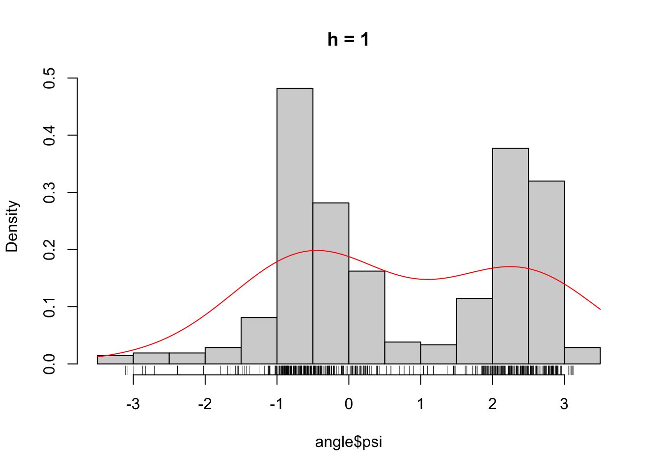
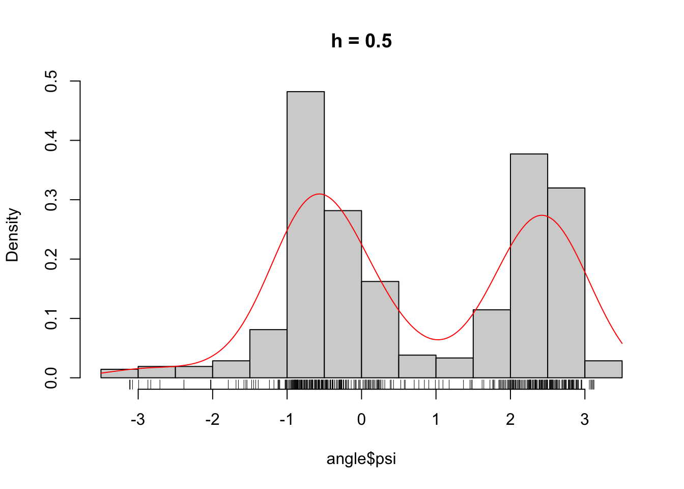
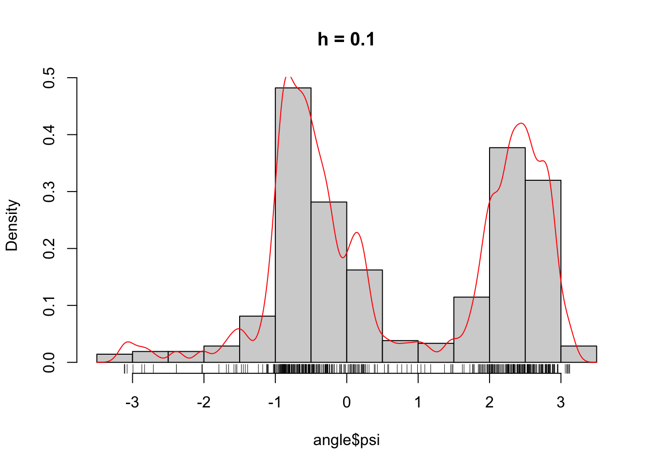
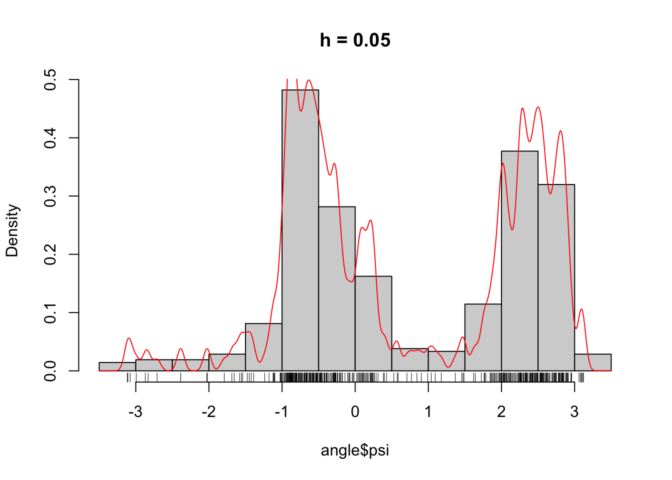
Figure 2.6: The densities \(\overline{f}_h\) for different choices of \(h\).
The way that these densities adapt to the data points is reflected in the log-likelihood as well.
hseq <- seq(1, 0.001, -0.001)
ll <- sapply(hseq, function(h) sum(log(f_bar(angle$psi, h))))
ggplot(mapping = aes(hseq, ll)) + geom_line() +
  xlab("h") + ylab("Log-likelihood")
ggplot(mapping = aes(hseq, ll)) + geom_line() +
  scale_x_log10("h (log-scale)") + ylab("")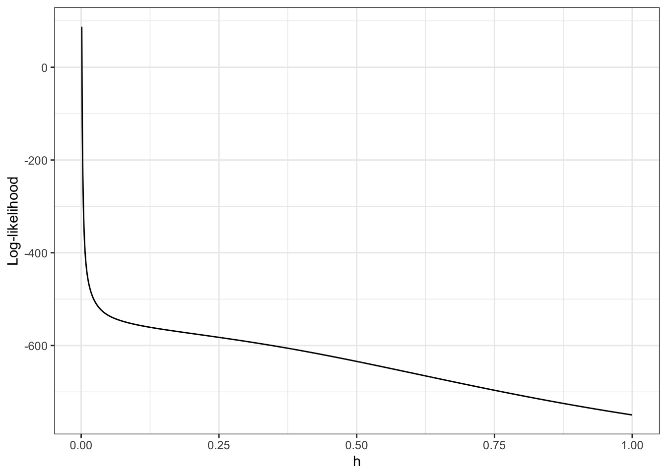
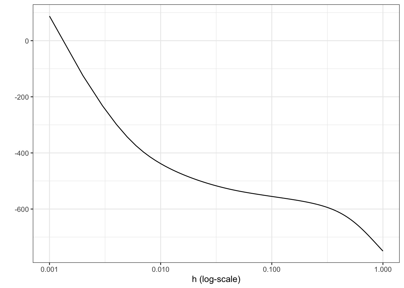
Figure 2.7: Log-likelihood, \(\ell(\overline{f}_h)\), for the densities \(\overline{f}_h\) as a function of \(h\). Note the log-scale on the right.
From Figure 2.7 it is clear that the likelihood is decreasing in \(h\), and it appears that it is unbounded as \(h \to 0\). This is most clearly seen on the figure when \(h\) is plotted on the log-scale because then it appears that the log-likelihood approximately behaves as \(-\log(h)\) for \(h \to 0\).
We can show that that is, indeed, the case. If \(x_i \neq x_j\) when \(i \neq j\)
\[\begin{align*} \ell(\overline{f}_h) & = \sum_{i} \log\left(1 + \sum_{j \neq i} e^{-(x_i - x_j)^2 / (2 h^2)} \right) - n \log(nh\sqrt{2 \pi}) \\ & \sim - n \log(nh\sqrt{2 \pi}) = - n \log(h) - n \log(n\sqrt{2 \pi}) \end{align*}\]
for \(h \to 0\). Hence, \(\ell(\overline{f}_h) \to \infty\) for \(h \to 0\). This demonstrates that the maximum-likelihood estimator of the density does not exist in the set of all distributions with densities.
In the sense of weak convergence it actually holds that
\[ \overline{f}_h \cdot m \overset{\mathrm{wk}}{\longrightarrow} P_N = \frac{1}{N} \sum_{j=1}^N \delta_{x_j} \]
for \(h \to 0\). The empirical measure \(P_N\) can sensibly be regarded as a nonparametric maximum-likelihood estimator of the distribution, but the empirical measure does not have a density. We conclude that we cannot directly define a sensible density estimator as a maximum-likelihood estimator.
2.3.1 Basis expansions
We suppose in this section that the data points are all contained in the interval \([a,b]\) for \(a, b \in \mathbb{R}\). This is true for the angle data with \(a = -\pi\) and \(b = \pi\) no matter the size of the dataset, but if \(f_0\) does not have a bounded support it may be necessary to let \(a\) and \(b\) change with the data. However, for any fixed dataset we can choose some sufficiently large \(a\) and \(b\).
Suppose that we have chosen \(p\) continuous functions \(\varphi_1, \ldots, \varphi_p : [a,b] \to \mathbb{R}\). These will be called basis functions. We then define the density
\[ f_{\boldsymbol{\beta}}(x) = \frac{1}{c(\boldsymbol{\beta})} \exp\left(\sum_{k=1}^p \beta_k \varphi_k(x)\right) \]
for the parameter \(\boldsymbol{\beta} = (\beta_1, \ldots, \beta_h)^T \in \mathbb{R}^p\). The normalization constant is
\[ c(\boldsymbol{\beta}) = \int_a^b \exp\left(\sum_{k=1}^p \beta_k \varphi_k(x)\right) \mathrm{d} x. \]
The maximum-likelihood estimator is then
\[\begin{align*} \hat{\boldsymbol{\beta}} & = \argmax_{\boldsymbol{\beta} \in \mathbb{R}^p} \ \sum_{j=1}^N \left(\sum_{k=1}^p \beta_k \varphi_k(x_j) \right) - \log c(\boldsymbol{\beta}) \\ & = \argmax_{\boldsymbol{\beta} \in \mathbb{R}^p} \ \ \mathbf{1}^T \boldsymbol{\Phi} \boldsymbol{\beta} - N \log c(\boldsymbol{\beta}). \end{align*}\]
Here \(\boldsymbol{\Phi}\) is the \(N \times p\) matrix with \(\boldsymbol{\Phi}_{jk} = \varphi_k(x_j)\). By differentiation, the maximum-likelihood estimator is seen to be a solution to the non-linear equation
\[\begin{equation} \mathbf{1}^T \boldsymbol{\Phi} = N \tau(\boldsymbol{\beta}) \end{equation}\]
where \(\tau : \mathbb{R}^p \to \mathbb{R}^p\) is the map with coordinates
\[ \tau_l(\boldsymbol{\beta}) = \frac{\partial_l c(\boldsymbol{\beta})}{c(\boldsymbol{\beta})} = \frac{1}{c(\boldsymbol{\beta})} \int_a^b \varphi_l(x) \exp\left(\sum_{k=1}^p \beta_k \varphi_k(x)\right) \mathrm{d} x \]
for \(l \in \{1, \ldots, p\}\). It may not be entirely straightforward how to compute \(c(\boldsymbol{\beta})\), but it is possible to implement the computation of \(\tau\) using numerical integration, and the equation above can then be solved numerically as well. We will, however, pursue a different estimation technique that does not require numerical evaluation of integrals or solving non-linear equations.
2.3.2 Score matching
Suppose that the basis functions are twice differentiable and define the \(p \times p\) matrix \(\mathbf{B}\) and the \(p\)-vector \(\mathbf{b}\) by
\[\begin{align*} \mathbf{B}_{kl} & = \sum_{j=1}^N \phi_k'(x_j) \phi_l'(x_j) \\ \mathbf{b}_k & = \sum_{j=1}^N \phi_k''(x_j). \end{align*}\]
If \(\mathbf{B}\) is of full rank \(p\), the score matching estimator equals
\[ \tilde{\boldsymbol{\beta}} = \mathbf{B}^{-1} \mathbf{b}. \]
The score matching estimator is simple to define and compute by the expression above, which involves only the evaluations of the two first derivatives of the basis functions in the data points and a single solution of a linear equation in \(p\) unknowns. The justification of the score matching estimator is a little more involved, and it involves a boundary assumption, which we will return to.
Assuming the basis functions and \(f_0\) are continuously differentiable we define the Fisher divergence as
\[ J(\boldsymbol{\beta}) = \int_a^b \left( \frac{f_0'(x)}{f_0(x)} - \frac{f_{\boldsymbol{\beta}}'(x)}{f_{\boldsymbol{\beta}}(x)}\right)^2 f_0(x) \mathrm{d}x. \]
The best approximation of \(f_0\) in terms of the Fisher divergence is found by minimizing \(J(\boldsymbol{\beta})\). To derive an estimator we rewrite \(J(\boldsymbol{\beta})\) as follows
\[\begin{align*} J(\boldsymbol{\beta}) & = \int_a^b \left( \frac{f_0'(x)}{f_0(x)} \right)^2 f_0(x) \mathrm{d}x + \int_a^b \left( \frac{f_{\boldsymbol{\beta}}'(x)}{f_{\boldsymbol{\beta}}(x)} \right)^2 f_0(x) \mathrm{d}x + \\ & \qquad 2 \int_a^b \left(\frac{f_{\boldsymbol{\beta}}'(x)}{f_{\boldsymbol{\beta}}(x)} \right) \left( \frac{f_0'(x)}{f_0(x)} \right) f_0(x) \mathrm{d}x \\ & = C(f_0) + \int_a^b \left( \sum_{k=1}^p \beta_k \phi_k'(x) \right)^2 f_0(x) \mathrm{d}x + 2 \int_a^b \left( \sum_{k=1}^p \beta_k \phi_k'(x) \right) f_0'(x) \mathrm{d}x. \end{align*}\]
The first term above does not depend on the parameter \(\boldsymbol{\beta}\), and the second term is an expectation, which can be estimated by
\[ \frac{1}{N} \sum_{j=1}^N \left(\sum_{k=1}^p \beta_k \phi_k'(x_j) \right)^2 = \frac{1}{N} \boldsymbol{\beta}^T \mathbf{B} \boldsymbol{\beta} \]
where \(\mathbf{B}\) is a symmetric and positive semi-definite matrix. To estimate the third term above we use integration-by-parts, which gives
\[ \int_a^b \left( \sum_{k=1}^p \beta_k \phi_k'(x) \right) f_0'(x) \mathrm{d}x = \left( \sum_{k=1}^p \beta_k \phi_k'(x) \right) f_0(x) \Bigg|_a^b - \int_a^b \left( \sum_{k=1}^p \beta_k \phi_k''(x) \right) f_0(x) \mathrm{d}x \]
assuming that the basis functions are twice continuously differentiable. If
- either \(f_0(a) = f_0(b) = 0\)
- or \(f_0(a) = f_0(b)\) together with \(\phi_k''(a) = \phi_k''(b)\) for \(k = 1, \ldots, p\)
the first term above vanishes, and we can estimate the second term as an expectation by
\[ \frac{1}{N} \sum_{j=1}^N \sum_{k=1}^p \beta_k \phi_k''(x_j) = \frac{1}{N} \mathbf{b} \boldsymbol{\beta} \]
where
\[ \tilde{\boldsymbol{\beta}} = \argmin_{\boldsymbol{\beta}} \tilde{J}(\boldsymbol{\beta}) \]
where the empirical objective function we minimize is the quadratic function
\[ \tilde{J}(\boldsymbol{\beta}) = \boldsymbol{\beta}^T \mathbf{B} \boldsymbol{\beta} - 2 \mathbf{b} \boldsymbol{\beta} \]
When \(\mathbf{B}\) has full rank, the unique minimizer and score matching estimator is given explicitly as
Many basis functions are possible. One possible choice is the trigonometric functions
\[ \varphi_1(x) = \cos(x), \varphi_2(x) = \sin(x), \ldots, \varphi_{2p-1}(x) = \cos(hx), \varphi_{2p}(x) = \sin(hx) \]
on the interval \([-\pi, \pi]\). In Section 1.2.1 a simple special case was actually treated corresponding to \(p = 2\), where the normalization constant was identified in terms of a modified Bessel function.
John von Neumann is famously quoted for saying that “With four parameters I can fit an elephant, and with five I can make him wiggle his trunk.” An example of a four-parameter family of distributions is the normal-inverse Gaussian distributions with the generalized hyperbolic distributions an extension with five parameters. These are flexible distributions, with the parameters controlling scale and location of the distribution, and additional shape properties such as tail decay and (a)symmetry. However, von Neumann was probably thinking more in terms of expansions with four or five suitably chosen basis functions, such as the trigonometric functions above, or using polynomials or splines as will be treated in more detail in Sections 3.5.1 and 3.5. What his quote says is that even with relatively few parameters we can adapt a basis expansion so that approximates many functions quite well. With too many parameters, we easily end up overfitting the model to data. That is, we adapt the model too much to the individual data points in the dataset, in which case it is not a good representation of the underlying distribution.
The quote is not a mathematical statement but an empirical observation. With a handful of parameters we get a quite flexible class of densities that will fit many real datasets well. But remember that a reasonably good fit does not mean that we have found the “true” data generating model. Though data is in some situations not as scarce a resource today as when von Neumann made elephants wiggle their trunks, the quote suggests that \(h\) should grow rather slowly with \(N\) to avoid overfitting.
2.3.3 Method of sieves
A sieve is a family of models, \(\Theta_{h}\), indexed by a real valued parameter, \(h \in \mathbb{R}\), such that \(\Theta_{h_1} \subseteq \Theta_{h_2}\) for \(h_1 \leq h_2\). In this chapter \(\Theta_{h}\) will denote a set of probability densities. If the increasing family of models is chosen in a sensible way, we may be able to compute the maximum-likelihood estimator
\[ \hat{f}_h = \argmax_{f \in \Theta_h} \ell(f), \]
and we may even be able to choose \(h = h_N\) as a function of the sample size \(n\) such that \(\hat{f}_{h_N}\) becomes a consistent estimator of \(f_0\).
It is possible to take
\[ \Theta_h = \{ \overline{f}_{h'} \mid h' \leq h \} \]
with \(\overline{f}_{h'}\) as defined above, in which case \(\hat{f}_h = \overline{f}_h\). We will see in the following section that this is simply a kernel estimator.
A more interesting example is obtained by letting
\[ \Theta_h = \left\{ x \mapsto \frac{1}{h \sqrt{2 \pi}} \int e^{- \frac{(x - z)^2}{2 h^2} } \mathrm{d}\mu(z) \Biggm| \mu \textrm{ a probability measure} \right\}, \]
which is known as the convolution sieve. We note that \(\overline{f}_h \in \Theta_h\) by taking \(\mu = \P_N\), but generally \(\hat{f}_h\) will be different from \(\overline{f}_h\).
We will not pursue the general theory of sieve estimators, but refer to the paper Nonparametric Maximum Likelihood Estimation by the Method of Sieves by Geman and Hwang. In the following section we will work out some more practical details for a particular sieve estimator based on a basis expansion of the log-density.
2.4 Cross-validation
An alternative to relying on the asymptotic optimality arguments for integrated mean squared error and the corresponding plug-in estimates of the bandwidth is known as cross-validation. The method mimics the idea of setting aside a subset of the dataset, which is then not used for computing an estimate but only for validating the estimator’s performance. The benefit of cross-validation over simply setting aside a validation dataset is that we do not “waste” any of the data points on validation only. All data points are used for the ultimate computation of the estimate. The deficit is that cross-validation is usually computationally more demanding.
Suppose that \(I_1, \ldots, I_k\) form a partition of the index set \(\{1, \ldots, N\}\) and define
\[ I^{-i} = \bigcup_{l: i \not \in I_l} I_l. \]
That is, \(I^{-i}\) contains all indices but those that belong to the set \(I_l\) containing \(i\). In particular, \(i \not \in I^{-i}\). Define also \(N_i = |I^{-i}|\) and
\[ \hat{f}^{-i}_h = \frac{1}{h N_i} \sum_{j \in I^{-i}} K\left(\frac{x_i - x_j}{h}\right). \]
That is, \(\hat{f}^{-i}_h\) is the kernel density estimate based on data with indices in \(I^{-i}\) and evaluated in \(x_i\). Since the density estimate evaluated in \(x_i\) is not based on \(x_i\), the quantity \(\hat{f}^{-i}_h\) can be used to assess how well the density estimate computed using a bandwidth \(h\) concur with the data point \(x_i\). This can be summarized using the log-likelihood
\[ \ell_{\mathrm{CV}}(h) = \sum_{i=1}^N \log (\hat{f}^{-i}_h), \]
that we will refer to as the cross-validated log-likelihood, and we define the bandwidth estimate as
\[ \hat{h}_{\mathrm{CV}} = \argmax_h \ \ \ell_{\mathrm{CV}}(h). \]
This cross-validation based bandwidth can then be used for computing kernel density estimates using the entire dataset.
If the partition of indices consists of \(k\) subsets we usually talk about \(k\)-fold cross-validation. If \(k = n\) so that all subsets consist of just a single index we talk about leave-one-out cross-validation. For leave-one-out cross-validation there is only one possible partition, while for \(k < n\) there are many possible partitions. Which should be chosen then? In practice, we choose the partition by sampling indices randomly without replacement into \(k\) sets of size roughly \(n / k\).
It is also possible to use cross-validation in combination with MISE. Rewriting we find that
\[ \mathrm{MISE}(h) = E (\| \hat{f}_h\|_2^2) - 2 E (\hat{f}_h(X)) + \E(\|f_0^2\|_2^2) \]
for \(X\) a random variable independent of the data and with distribution having density \(f_0\). The last term does not depend upon \(h\) and we can ignore it from the point of view of minimizing MISE. For the first term we have an unbiased estimate in \(\| \hat{f}_h\|_2^2\). The middle term can be estimated without bias by
\[ \frac{2}{N} \sum_{i=1}^N \hat{f}^{-i}_h, \]
and this leads to the statistic
\[ \mathrm{UCV}(h) = \| \hat{f}_h\|_2^2 - \frac{2}{N} \sum_{i=1}^N \hat{f}^{-i}_h \]
known as the unbiased cross-validation criterion. The corresponding bandwidth estimate is
\[ \hat{h}_{\mathrm{UCV}} = \textrm{arg min}_h \ \ \mathrm{UCV}(h). \]
Contrary to the log-likelihood based criterion, this criterion requires
the computation of \(\| \hat{f}_h\|_2^2\). Bandwidth selection using UCV
is implemented in R in the function bw.ucv() and can be
used with density() by setting the argument bw = "ucv".
2.5 Exercises
Exercise 2.1 The Epanechnikov kernel is given by
\[ K(x) = \frac{3}{4}(1 - x^2) \]
for \(x \in [-1, 1]\) and 0 elsewhere. Show that this is a probability density with mean zero and compute \(\sigma_K^2\) as well as \(\|K\|_2^2\).
For the following exercises use the log(F12) variable as considered in Exercise A.4.
Exercise 2.2 Use density() to compute the kernel density estimate with the Epanechnikov kernel
to the log(F12) data. Try different bandwidths.
Exercise 2.3 Implement kernel density estimation yourself using the Epanechnikov kernel.
Test your implementation by comparing it to density() using the log(F12) data.
Exercise 2.4 Construct the following vector
x <- rnorm(2^13)Then use bench::mark() to benchmark the computation of
density(x[1:k], 0.2)for k ranging from \(2^5\) to \(2^{13}\). Summarize the benchmarking results.
Exercise 2.5 Benchmark your own implementation of kernel density estimation using the Epanechnikov
kernel. Compare the results to those obtained for density().
Exercise 2.6 Experiment with different implementations of kernel evaluation in R using
the Gaussian kernel and the Epanechnikov kernel. Use bench::mark() to compare
the different implementations.