\(\DeclareMathOperator*{\argmin}{argmin}\) \(\DeclareMathOperator*{\argmax}{argmax}\) \(\newcommand{\E}{\mathbf{E}}\) \(\newcommand{\V}{\mathbf{Var}}\) \(\newcommand{\cov}{\mathbf{Cov}}\) \(\newcommand{\P}{\mathbf{P}}\)

3 Scatterplot smoothing

This chapter is on the estimation of a smooth relation between a real valued variable \(Y\) an another variable \(X\). We will mostly consider \(X\) to be real valued as well, in which case a first impression of their relation is obtained from data \((x_1, y_1), \ldots, (x_N, y_N)\) by a scatterplot of \(y_i\) against \(x_i\). Our aim is essentially to smooth the relation that the scatterplot shows, hence the term “scatterplot smoothing”.

We will throughout this chapter use a temperature dataset from Greenland. The raw data is available from the site SW Greenland temperature data, but data is also included in the CSwR package. See, in addition, (Vinther et al. 2006).

head(greenland)

##   Year Month Temp_nuuk Temp_Qaqortoq Temp_diff
## 1 1873     1     -12.1          -9.9      -2.2
## 2 1874     1     -13.1         -11.6      -1.5
## 3 1875     1      -6.6          -6.3      -0.3
## 4 1876     1     -11.1          -8.3      -2.8
## 5 1877     1     -14.5          -8.8      -5.7
## 6 1878     1      -7.7          -6.8      -0.9

The greenland dataset contains monthly average temperatures in degree Celsius from 1873 to 2013 in Nuuk and Qaqortoq, a town south of Nuuk in Greenland. The last column contains the temperature difference (temperature in Nuuk minus temperature in Qaqortoq). We plot the temperature difference (\(Y\)) against the temperature in Qaqortoq (\(X\)).

p_greenland <- ggplot(greenland, aes(Temp_Qaqortoq, Temp_diff)) + 
  geom_point(shape = 16, alpha = 0.3) + 
  xlab("Temperature Qaqortoq") +
  ylab("Temperature difference") +
  geom_line(aes(y = mean(Temp_diff)), linetype = 2, linewidth = 1)
p_greenland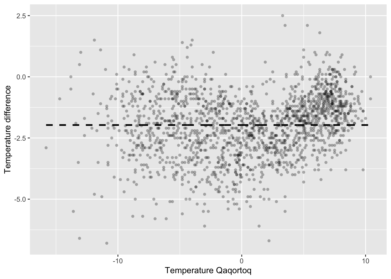

Figure 3.1: Monthly temperature difference between Nuuk and Qaqortoq plottet against the temperature in Qaqortoq. The dashed horizontal line is the average temperature difference.

The scatterplot in Figure 3.1 shows that the temperature in Nuuk is about \(2{\ }^{\circ}\mathrm{C}\) lower than in Qaqortoq on average, but that there are local variations. When it is warm, the temperature difference is smaller, but when it is about \(0{\ }^{\circ}\mathrm{C}\) in Qaqortoq, the difference is larger. A scatterplot smoother should capture such local variations.

Throughout this chapter we focus on estimation of (aspects of) the conditional distribution of \(Y\) given \(X\). Thus the variables are treated asymmetrically. We will mostly consider estimation of the function

\[ f(x) = \E(Y \mid X = x), \]

which is the conditional mean of \(Y\) given \(X = x\). For the temperature data, \(f(x)\) is the mean temperature difference given that the temperature in Qaqortoq is \(x {\ }^{\circ}\mathrm{C}\). The function \(f\) can be used to predict the temperature in Nuuk as \(x + f(x)\) in terms of the temperature \(x\) in Qaqortoq. The dashed horizontal line in Figure 3.1 is the simplest scatterplot smoother that assumes \(f\) is constant.

Another simpel example of a scatterplot smoother is a straight line, which we can fit using least squares. This is a useful smoother if \(f(x)\) is approximately an affine function. Letting

\[ \mathbf{X} = \left( \begin{array}{cc} 1 & x_1 \\ 1 & x_2 \\ \vdots & \vdots \\ 1 & x_N \end{array} \right) \]

denote the model matrix, the least squares straight line fit is given by \(\hat{f}(x) = \hat{\beta}_0 + \hat{\beta}_1 x\) with

\[ \left( \begin{array}{c} \hat{\beta}_0 \\ \hat{\beta}_1 \end{array} \right) = (\mathbf{X}^T \mathbf{X})^{-1} \mathbf{X}^T \mathbf{y} = \left( \begin{array}{cc} N & \sum_{i=1}^N x_i \\ \sum_{i=1}^N x_i & \sum_{i=1}^N x_i^2 \end{array} \right)^{-1} \left( \begin{array}{c} \sum_{i=1}^N y_i \\ \sum_{i=1}^N x_iy_i \end{array} \right). \]

The fitted values are denoted \(\hat{f}_i = \hat{f}(x_i) = \hat{\beta}_0 + \hat{\beta}_1 x_i\), and we see that the vector of fitted values is given as

\[ \hat{\mathbf{f}} = \mathbf{X}^T \left( \begin{array}{c} \hat{\beta}_0 \\ \hat{\beta}_1 \end{array} \right) = \mathbf{X}^T (\mathbf{X}^T \mathbf{X})^{-1} \mathbf{X}^T \mathbf{y}. \]

We often consider a scatterplot smoother as a mapping determined by the \(x_i\)-s that map the observed values, \(\mathbf{y}\), to the fitted (or predicted) values, \(\hat{\mathbf{f}}\). Least squares defines such a mapping as given above. It is a linear mapping. Any smoother that, for fixed \(x_i\)-s, results in a linear mapping

\[\begin{equation} \mathbf{y} \mapsto \hat{\mathbf{f}} = \mathbf{S} \mathbf{y} \tag{3.1} \end{equation}\]

of observed values to fitted values is called a linear smoother. The matrix \(\mathbf{S}\), representing the linear map, is called the smoother matrix. The least squares straight line smoother has smoother matrix \(\mathbf{S} = \mathbf{X}^T (\mathbf{X}^T \mathbf{X})^{-1} \mathbf{X}^T\).

Some scatterplot smoothers are very easy to add to the ggplot2 objects via the geom_smooth() function, and two examples are demonstrated below.

p_greenland +
  geom_smooth(
    method = "lm", 
    formula = y ~ x,                 # The straight line smoother
    se = FALSE,
    color = "purple"
  ) +
   geom_smooth(
    method = "gam",                  
    formula = y ~ s(x, bs = "cr"),   # A spline smoother
    se = FALSE
  )

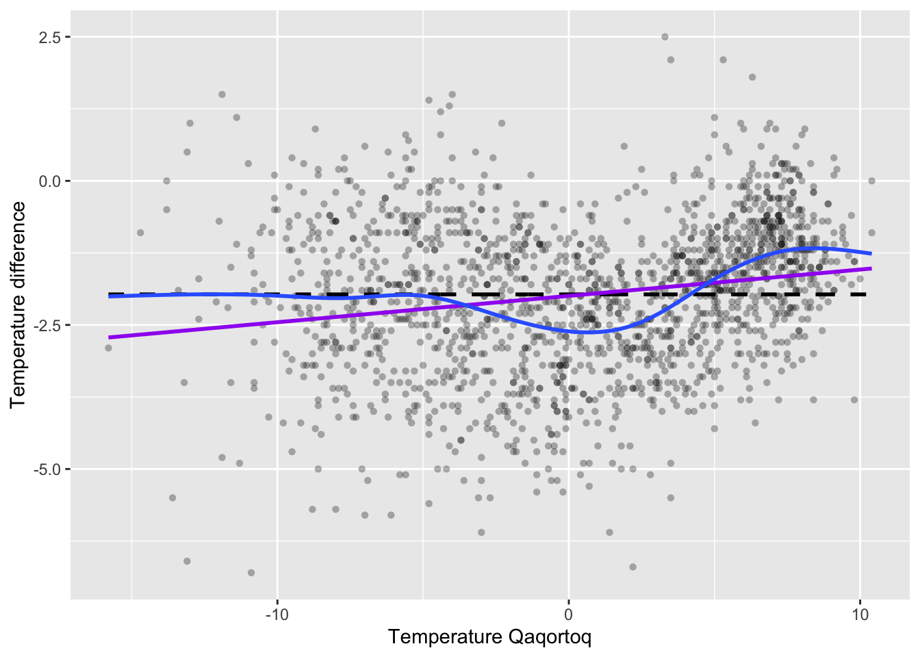
Figure 3.2: Monthly temperature difference between Nuuk and Qaqortoq plottet against the temperature in Qaqortoq. The horizontal dashed line is the average temperature difference, and the straight line smoother (purple) and a spline smoother (blue) are added.

Figure 3.1 shows the scatterplot of the temperature data with the straight line smoother and a spline smoother added. The spline smoother captures the nonlinear local variations from the horizontal line well.

3.1 Nadaraya–Watson kernel smoothing

The straight line smoother obtained by least squares, as in Figure 3.2, is a global smoother. Two parameters are estimated to optimize a global measure of how well the line fits the data. It does not capture the local variations in the data well. The spline smoother included in Figure 3.2 can also be considered a global smoother but using a flexible model based on a basis expansion. We return to those smoothers in Section 3.5. In this section we consider local smoothers.

A local smoother focuses on fitting models in neighborhoods of the \(x_i\)-s. Supposing that \(B_i\) is a neighborhood of \(x_i\) for each \(i = 1, \ldots, N\), a simple smoother is given by

\[ \hat{f}_i = \frac{\sum_{j=1}^N y_j 1_{B_i}(x_j)}{\sum_{j=1}^N 1_{B_i}(x_j)}. \]

That is, \(\hat{f}_i\) is simply the average of the \(y_j\)-s for which the corresponding \(x_j\)-s fall in the neighborhood \(B_i\) of \(x_i\). This local smoother regards \(f\) as approximately constant in the neighborhoods of the \(x_i\)-s. Note that \(\hat{f}_i\) can be defined for \(x_i\)-values in a quite general space; they do not need to be real numbers, we just need a way to define what we mean by “neighborhood”.

In a metric space the natural choice of \(B_i\) is the ball, \(B(x_i, h)\), around \(x_i\) with some radius \(h\). In \(\mathbb{R}\) with the usual metric (or even \(\mathbb{R}^p\) equipped with any norm-induced metric) we have that

\[ 1_{B(x_i, h)}(x) = 1_{B(0, 1)}\left(\frac{x - x_i}{h}\right), \]

thus since \(B(0, 1) = [-1, 1]\) in \(\mathbb{R}\),

\[ \hat{f}_i = \frac{\sum_{j=1}^N y_j 1_{[-1, 1]}\left(\frac{x_j - x_i}{h}\right)}{\sum_{l=1}^N 1_{[-1, 1]}\left(\frac{x_l - x_i}{h}\right)}. \]

This nonparametric estimator of the conditional mean \(f(x_i)\) is closely related to the kernel density estimator with the rectangular kernel, see Section 2.1, and just as for that estimator there is a natural generalization allowing for arbitrary kernels instead of the indicator function \(1_{[-1, 1]}\).

With \(K : \mathbb{R} \mapsto \mathbb{R}\) a fixed kernel the corresponding kernel smoother with bandwidth \(h\) becomes

\[ \hat{f}_i = \frac{\sum_{j=1}^N y_j K\left(\frac{x_j - x_i}{h}\right)}{\sum_{l=1}^N K\left(\frac{x_l - x_i}{h}\right)}. \]

This smoother is known as the Nadaraya–Watson kernel smoother or Nadaraya–Watson estimator. See Exercise 3.1 for an additional perspective based on bivariate kernel density estimation.

The Nadaraya–Watson kernel smoother is a linear smoother with smoother matrix \(\mathbf{S}\) with entries

\[ S_{ij} = \frac{K\left(\frac{x_j - x_i}{h}\right)}{\sum_{l=1}^N K\left(\frac{x_l - x_i}{h}\right)}. \]

The Nadaraya–Watson kernel smoother can be implemented in much the same way as the kernel density estimator, and the runtime will inevitably scale like \(O(N^2)\) unless we exploit special properties of the kernel or use approximation techniques. We implement the kernel smoother with the Gaussian kernel as a linear estimator and using the function outer() to compute \(\mathbf{S}\).

kern_smooth <- function(x, y, h) {
  K <- outer(x, x, function(x1, x2) exp(-(x1 - x2)^2 / (2 * h^2)))
  S <- K / rowSums(K)
  S %*% y
}

We can then apply kernel smoothing to the temperature data.

f_hat <- kern_smooth(
  greenland$Temp_Qaqortoq, 
  greenland$Temp_diff,
  h = 0.5
)

p_greenland + 
  geom_line(aes(y = f_hat), color = "blue", lwd = 1)

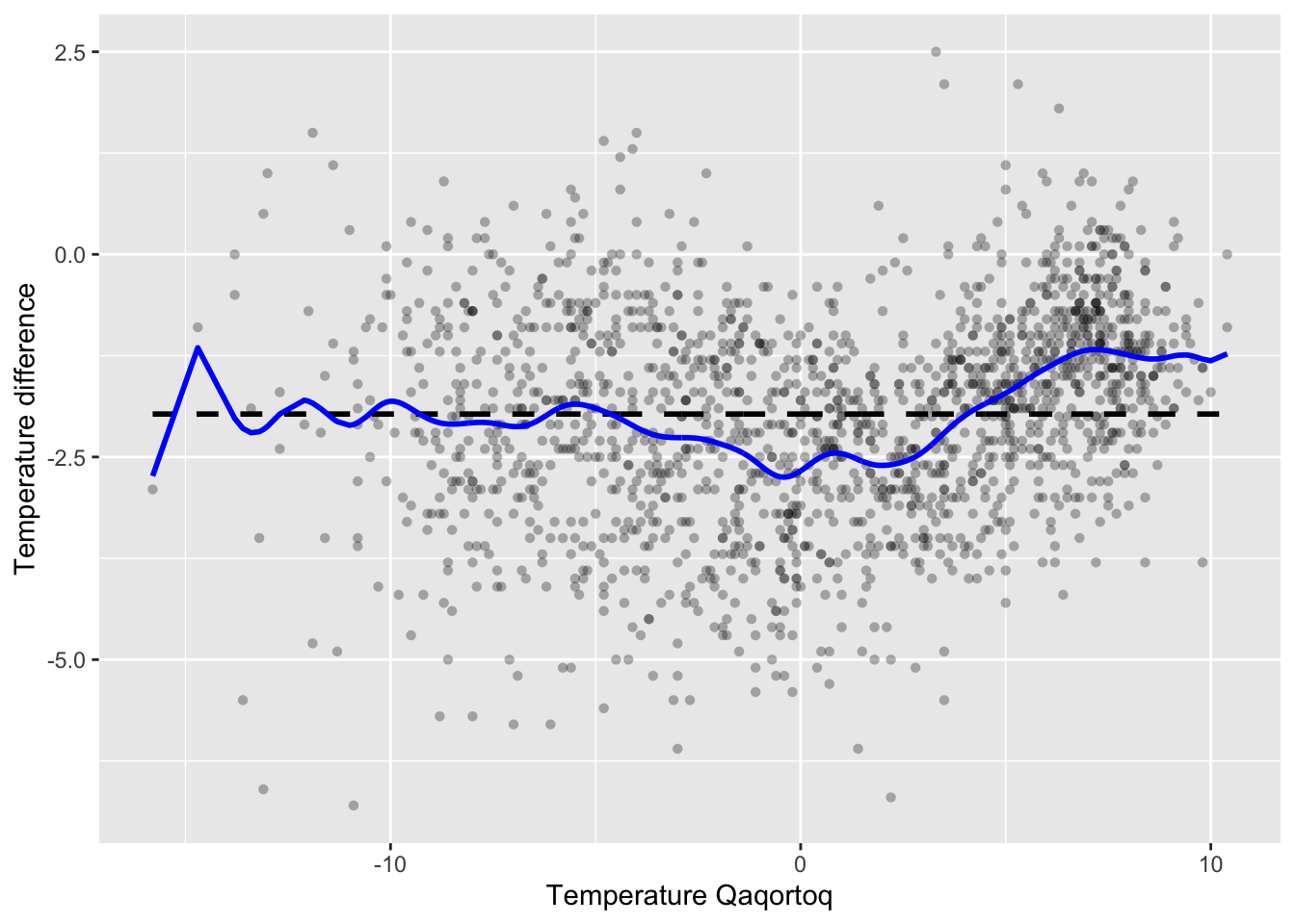
Figure 3.3: Nadaraya–Watson kernel smoother of temperature difference between Nuuk and Qaqortoq computed using the smoother matrix and the Gaussian kernel with bandwidth 0.5.

Basic kernel smoothing is also implemented in the ksmooth() function from the stats package. To test our implementation we compare the result on the temperature data to the result from ksmooth(). This is slightly tricky beause ksmooth() internally rescales the bandwidth to make the kernel have quartiles in \(\pm 0.25 h\) (see ?ksmooth). For the Gaussian kernel the rescaling amounts to multiplying \(h\) by the factor \(0.3706506\).

f_hat_ksmooth <- ksmooth(
  greenland$Temp_Qaqortoq, 
  greenland$Temp_diff, 
  kernel = "normal",
  bandwidth = 0.5 /  0.3706506,  # ksmooth() rescales!
  x.points = greenland$Temp_Qaqortoq
)
ord <- order(greenland$Temp_Qaqortoq)
range(f_hat[ord] - f_hat_ksmooth$y)

## [1] -1.517e-04  7.929e-05

The comparison shows that the differences are small but still of the order \(10^{-5}\), which is larger than can be explained by rounding errors alone. In fact, ksmooth() truncates the tails of the Gaussian kernel to 0 beyond \(4h\). This is where the kernel becomes less than \(0.000335 \times K(0) = 0.000134\), which for practical purposes is zero. The truncation explains the relatively large differences between the two implementations that should otherwise be equivalent. It is an example where the approximate solution computed by ksmooth() is acceptable because the truncation results in substantial reduction of runtime.

3.2 Leave-one-out cross-validation

Cross-validation was introduced in Section 2.4 as a method for assessing the performance of a model. In the context of scatterplot smoothing, we can assess performance by measuring how well the model predicts out-of-sample. That is, how well \(y_i\) is predicted from \(x_i\) for data points \((x_i, y_i)\) not in the dataset used for computing the smoother. In this section we focus on leave-one-out cross-validation where the prediction for each data point is based on a smoother using all other data but that point.

In many cases a smoother has a natural definition of an out-of-sample prediction, that is, how \(\hat{f}(x)\) is computed for \(x\) not in the data. If so, it is possible to define

\[ \hat{f}^{-i}_i = \hat{f}^{-i}(x_i) \]

as the prediction at \(x_i\) using the smoother computed from data with \((x_i, y_i)\) excluded. Formulas or methods for out-of-sample prediction do, however, generally depend on the specific smoother used. For a linear smoother with smoother matrix \(\mathbf{S}\) we will define the leave-one-out prediction as

\[ \hat{f}^{-i}_i = \sum_{j \neq i} \frac{S_{ij}y_j}{1 - S_{ii}}. \]

This definition concurs with the out-of-sample predictor in \(x_i\) for most linear smoothers, but this has to be verified case-by-case.

Using the definition above, the leave-one-out cross-validation squared error criterion equals

\[ \mathrm{LOOCV} = \frac{1}{N} \sum_{i=1}^N (y_i - \hat{f}^{-i}_i)^2 = \frac{1}{N} \sum_{i=1}^N \left(\frac{y_i - \hat{f}_i}{1 - S_{ii}}\right)^2. \]

The important observation from the identity above is that \(\mathrm{LOOCV}\) can be computed without actually computing all the \(\hat{f}^{-i}_i\).

We will illustrate the use of leave-one-out cross-validation for bandwidth selection for the kernel smoother. Note that the diagonal elements of the smoother matrix are given as

\[ S_{ii} = \frac{K(0)}{\sum_{l=1}^N K\left(\frac{x_l - x_i}{h}\right)}. \]

The implementation below consists of two functions. One general function computes \(\mathrm{LOOCV}\) from the three ingredients: \(\mathbf{y}\), \(\hat{\mathbf{f}}\) and the vector of diagonal elements of \(\mathbf{S}\). The loocv_kern_smooth() function, specific to kernel smoothing with the Gaussian kernel, applies the general function to a grid of bandwidth parameters.

loocv_error <- function(y, f_hat, diag_S) {
  mean(((y - f_hat) / (1 - diag_S))^2) 
}

loocv_kern_smooth <- function(x, y, h) {
  logK <- outer(x, x, function(x1, x2) - (x1 - x2)^2 / 2)
  error <- function(h) {
     K <- exp(logK / h^2)
     S <- K / rowSums(K)
     loocv_error(y, S %*% y, diag(S))
  }
  sapply(h, error)
}

The implementation above can easily be made to work with any kernel and any sequence of \(x\)-s. Exercise 3.2 explores how to exploit symmetry of the kernel and equidistance of the \(x\)-s for efficient computation of the smoother matrix as well as the diagonal elements of the smoother matrix.

hs <- seq(0.2, 3, 0.05)
CV <- loocv_kern_smooth(greenland$Temp_Qaqortoq, greenland$Temp_diff, hs)
h_opt <- hs[which.min(CV)]
f_hat_opt <- kern_smooth(greenland$Temp_Qaqortoq, greenland$Temp_diff, h_opt)
ggplot(mapping = aes(hs, CV)) + geom_point() +
  geom_vline(xintercept = h_opt, color = "red")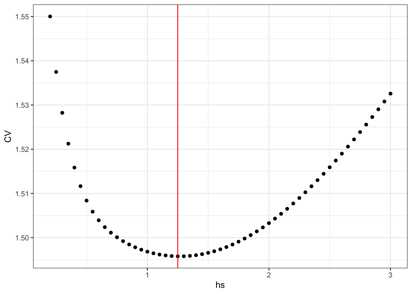

Figure 3.4: The leave-one-out cross-validation criterion for the kernel smoother using the Gaussian kernel as a function of the bandwidth \(h\).

The optimal bandwith is 1.25. We compute the resulting optimal smoother and compare it to the smoother computed using kern_smooth().

p_greenland + 
  geom_line(aes(y = f_hat_opt), color = "blue", linewidth = 1)

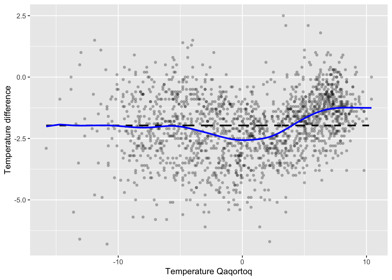
Figure 3.5: Nadaraya–Watson kernel smoother of the annual average temperature in Nuuk for the optimal bandwidth using LOOCV (blue) compared to the \(k\)-nearest neighbor smoother with \(k = 9\) (red).

Figure 3.5 shows the optimal kernel smoother. We note that the optimal bandwidth 1.25 results in a somewhat smoother curve than the bandwidth 0.5 that we initially considered.

3.3 Gaussian processes

Though kernel smoothing is a quite intuitive local smoother, it is also ad hoc. A more principled approach to smoothing is based on Gaussian processes, which posits a model of the target function \(f\) that we try to estimate. We introduce in this section Gaussian processes as a framework that naturally leads to linear smoothing, and we touch on some computational aspects. We also briefly discuss how Gaussian processes leads to new ways of choosing kernels and tuning parameters as well, but we leave the implementations as exercises. In Section 4.3 we return to some computationally efficient Gaussian process smoothers and their implementations in the context of time series.

The Gaussian process model supposes that the observed \(x_i\)-s are fixed, and it consists of a model of the vector \(\mathbf{f} = (f(x_1), \ldots, f(x_N))\) and a conditional model of \(Y_1, \ldots, Y_N\) given \(\mathbf{f}\). For simplicity, we suppose also in this section that \(x_i \in \mathbb{R}\), but Gaussian processes could be defined on quite general spaces.

The distribution of \(\mathbf{f}\) is defined in terms of a positive definite kernel function \(K : \mathbb{R} \to \mathbb{R}\). This is a function satisfying that the symmetric matrix \(\mathbf{K}\) defined by

\[ \mathbf{K}_{i,j} = K(x_i - x_j) \]

is positive semi-definite for any \(x_1, \ldots, x_N\). For such a kernel we suppose that \(\mathbf{f} \sim \mathcal{N}(m(\mathbf{x}), \mathbf{K})\) for some \(m(\mathbf{x}) \in \mathbb{R}^N\). Note that this model specifies the covariance between the coordinates of \(\mathbf{f}\) as

\[ \cov(f(x_i), f(x_j)) = K(x_i - x_j). \]

The conditional distribution of \(\mathbf{Y}\) given \(\mathbf{f}\) is also Gaussian,

\[ \mathbf{Y} \mid \mathbf{f} \sim \mathcal{N}(\mathbf{f}, \sigma^2 I) \]

with \(\sigma^2 > 0\) the observation variance.

It follows that the joint distribution of \(\mathbf{f}\) and \(\mathbf{Y}\) is a multivariate Gaussian distribution,

\[ (\mathbf{f}, \mathbf{Y}) \sim \mathcal{N}\left(\left(\begin{array}{c} m(\mathbf{x}) \\ m(\mathbf{x}) \end{array}\right), \left(\begin{array}{cc} \mathbf{K} & \mathbf{K} \\ \mathbf{K} & \mathbf{K} + \sigma^2 I \end{array} \right) \right). \]

Hence

\[ \hat{\mathbf{f}} = E(\mathbf{f} \mid \mathbf{Y} = \mathbf{y}) = m(\mathbf{x}) + \mathbf{K} (\mathbf{K} + \sigma^2 I)^{-1} (\mathbf{y} - m(\mathbf{x})). \]

If \(m(\mathbf{x}) = 0\) the conditional mean is a linear smoother with smoother matrix

\[\begin{equation} \mathbf{S} = \mathbf{K} (\mathbf{K} + \sigma^2 I)^{-1} = (I + \sigma^2 \mathbf{K}^{-1} )^{-1}. \tag{3.2} \end{equation}\]

Since \(m(\mathbf{x})\) is the mean of \(\mathbf{Y}\), we can also estimate a non-zero \(m(\mathbf{x})\). Suppose \(m(\mathbf{x}) \in L \subseteq \mathbb{R}^N\), where \(L\) is a linear subspace of \(\mathbb{R}^N\), then if \(P\) denotes the orthogonal projection onto \(L\), \(\hat{m}(\mathbf{x}) = P \mathbf{y}\) is the least squares estimate of \(m(\mathbf{x})\). Plugging this estimate into the formula for the conditional mean gives the linear smoother

\[ \hat{\mathbf{f}} = \hat{m}(\mathbf{x}) + \mathbf{K} (\mathbf{K} + \sigma^2 I)^{-1} (\mathbf{y} - \hat{m}(\mathbf{x})) = \underbrace{(\mathbf{K} (\mathbf{K} + \sigma^2 I)^{-1}(I - P) + P)}_{\mathbf{S}} \mathbf{y}. \]

This is a linear smoother satisfying that \(\mathbf{S} m(\mathbf{x}) = m(\mathbf{x})\). The simplest example is when \(m(\mathbf{x})\) is assumed to have identical entries, in which case \(\hat{m}(\mathbf{x}) = \overline{y} \mathbf{1}\), where \(\overline{y} = \frac{1}{N} \sum_{i=1}^N y_i\).

For the rest of this section we assume that \(m(\mathbf{x}) = 0\), which in practice can be achieved by substracting an estimate of \(m(\mathbf{x})\), as described above, and applying the Gaussian process smoother to the residuals.

The Neumann series then gives the approximation

\[\begin{equation} \mathbf{S} = \mathbf{K} (\mathbf{K} + \sigma^2 I)^{-1} = (\sigma^2)^{-1} \mathbf{K} + o((\sigma^2)^{-1}) \approx (\sigma^2)^{-1} \mathbf{K} \tag{3.3} \end{equation}\]

valid for large \(\sigma^2\). In this case, the Gaussian process smoother is similar to Nadaraya–Watson kernel smoothing with kernel \(K\), except for the row normalization. The main practical effect of the difference in row normalization is that the Gaussian process smoother shrinks the smoothed values toward zero. The larger \(\sigma^2\) is, the more are the values shrunk. A related shrinkage effect is discussed in Section 3.5.2 in the context of smoothing splines.

To compute the Gaussian process smoother we need to know the observation variance \(\sigma^2\) and the covariance matrix \(\mathbf{K}\), which is determined entirely from the kernel function \(K\) and the \(x_i\)-s. From this information we could compute the smoother matrix \(\mathbf{S}\). However, to compute \(\hat{\mathbf{f}}\) from the observation \(\mathbf{y}\), then rather than computing \(\mathbf{S}\), we can compute the smoother by the following two-step procedure

• Solve the equation \((\mathbf{K} + \sigma^2 I) \tilde{\mathbf{y}} = \mathbf{y}\)
• Compute \(\hat{\mathbf{f}} = \mathbf{K} \tilde{\mathbf{y}}\).

The approximation (3.3) shows that for large \(\sigma^2\), \(\tilde{\mathbf{y}} \approx (\sigma^2)^{-1} \mathbf{y}\), and if we use this approximation, Gaussian process smoothing is computationally equivalent to Nadaraya-Watson kernel smoothing. But even including the pre-smoothing step of first computing \(\tilde{\mathbf{y}}\), the solution of the linear equation does not change the runtime complexity, since we avoid the computationally expensive matrix inversion.

Standard algorithms for solving the linear equation and for the matrix-vector multiplication have time complexity \(O(N^2)\). Without additional structure on \(\mathbf{K}\), Gaussian process smoothing scales with the sample size in the same way as Nadaraya-Watson kernel smoothing, and large scale applications would require approximations. In Section 4.3 we describe the Kalman smoother, where the kernel has special structure, and where the smoother can we computed with time complexity \(O(N)\).

The Gaussian process approach specifies a fully generative model of \(Y_1, \ldots, Y_N\). This can be exploited for choosing the kernel, including any parameters in the kernel, and the variance parameter \(\sigma^2\). Still supposing that \(m(\mathbf{x}) = 0\), the marginal distribution of \(\mathbf{Y}\) is \(\mathcal{N}(0, \mathbf{K} + \sigma^2 I)\), thus the marginal log-likelihood function is

\[ \ell(\mathbf{K}, \sigma^2) = - \frac{1}{2} \mathbf{y}^T (\mathbf{K} + \sigma^2 I)^{-1} \mathbf{y} - \frac{1}{2}\log |\mathbf{K} + \sigma^2 I| \]

where \(|\mathbf{K} + \sigma^2 I|\) denotes the determinant of the matrix. Since \(\mathbf{K}\) is determined by the kernel, we can maximize \(\ell\) over kernel parameters and \(\sigma^2\) to optimize how well the model fits the data. We will not pursue the details here, see Chapter 2 in (Rasmussen and Williams 2006). We note that maximizing \(\ell\) is an alternative to choosing tuning parameters to optimize predictive performance, e.g., via cross-validation. Exercise 3.3 explores the use of the marginal log-likelihood for choosing tuning parameters.

3.4 Nearest neighbor smoothers

Kernel smoothers, whether derived from Gaussian processes or from ad hoc arguments, use the kernel function \(K\) to define locality in the \(x\)-space. The way \(K(x)\) decays toward \(0\) as \(x\) becomes large—possibly controlled by a bandwidth parameter—determines how data points count toward the local weighted averages. A disadvantage of this approach is that the estimator has high variance in those parts of the \(X\)-space that contain no or few data points. For real valued \(X\), this is mostly a problem in the tails of the \(X\)-distribution.

To remedy the problem with a heterogeneous distribution of \(X\)-values, we can define neighborhoods in a data adaptive way, e.g., in terms of the \(k\)-nearest neighbors. This definition fixes the number of neighbors, \(k\), instead of the size of the neighborhood. The resulting smoother is still a linear smoother, somewhat similar to the Nadaraya-Watson kernel smoother with the rectangular kernel, but it is a bit more involved to determine the neighborhood of all the data points—in particular if we want a runtime efficient implementation.

Mathematically, the \(k\)-nearest neighbor smoother in \(x_i\) is defined as

\[\begin{equation} \hat{f}_i = \frac{1}{k} \sum_{j \in \mathcal{N}_i} y_j \tag{3.4} \end{equation}\]

where \(\mathcal{N}_i\) is the set of indices for the \(k\)-nearest neighbors of \(x_i\). For simplicity, we will also refer to the index set \(\mathcal{N}_i\) as the neighborhood of \(x_i\). This simple idea of averaging the \(k\)-nearest neighbors is actually very powerful. It works as long as the \(X\)-values lie in a metric space, and by letting \(k\) grow with \(N\) it is possible to construct consistent nonparametric estimators of \(f(x) = E(Y \mid X= x)\) under minimal assumptions. With \(X\)-values in \(\mathbb{R}^p\), say, Theorem 2 in (Devroye et al. 1994) gives a strong universal consistency result of \(k\)-nearest neighbor smoothing assuming only that \(\E|Y| < \infty\) and that \(k/N \to 0\) and \(k/\log(N) \to \infty\). However, a practical problem is that \(k\) must grow slowly in high dimensions, and the estimator is not a panacea.

The main computational challenge is to find the neighborhood \(\mathcal{N}_i\) for each \(i\). A general solution is to compute all distances from \(x_i\) to \(x_j\) for \(j = 1, \ldots, N\) and then (partially) sort these to find the \(k\) smallest distances. This works for values in a general metric space—with a runtime that scales like \(O(N^2)\). See Exercise 3.4 for an implementation of the smoother matrix using this general approach.

For values in \(\mathbb{R}\), the total order of the real numbers implies that the neighborhoods are always of the form

\[ \mathcal{N}_i = \{\mathrm{left}_i, \mathrm{left}_i + 1, \ldots, \mathrm{right}_i - 1, \mathrm{right}_i\} \]

where \(\mathrm{left}_i \leq i \leq \mathrm{right}_i\) and \(\mathrm{right}_i - \mathrm{left}_i + 1 = k\). We can, moreover, find these neighborhood boundaries, \(\mathrm{left}_i\) and \(\mathrm{right}_i\), by sorting the \(x\)-values and then starting from \(\mathrm{left}_1 = 1\) and \(\mathrm{right}_1 = \min\{k, N\}\) we can sequentially update the boundaries. This is implemented by the function knn_boundaries() below.

knn_boundaries <- function(x, k) {
  if (is.unsorted(x)) x <- sort(x)
  N <- length(x)
  left <- right <- numeric(N)
  l <- left[1] <- 1
  r <- right[1] <- min(k, N)
  for(i in seq_along(x)[-1]) {
    while (r + 1 <= N && x[i] - x[l] >= x[r + 1] - x[i]) {
      r <- r + 1
      l <- l + 1
    }
    left[i] <- l
    right[i] <- r
  }
  list(left = left, right = right)
}

The function first sorts the \(x\)-values if they are unsorted. Each step in the sequential update is done using a while-loop. In this loop, the boundaries are moved one position to the right as long as the current left boundary is further from \(x_i\) than the updated right boundary.

There is a subtle issue with ties. When multiple \(x\)-values are identical, the neighborhoods \(\mathcal{N}_i\), and thus their boundaries, are not uniquely defined. There are several possibilities for breaking ties, e.g., by randomization. This could be achieved by adding tiny amounts of i.i.d. random noise to the \(x_i\)-s. In the implementation of knn_boundaries() we implicitly let the sort() function determine how ties are handled. Consequently, the order of the data points in the dataset can also matter.

How ties are handled is mostly irrelevant for practical purposes—unless \(X\) only takes values in a discrete subset of \(\mathbb{R}\). But it is a nuisance that results depend on such arbitrary details. This is particularly so when we test our implementations, since we then need to make sure that different implementations handle ties in exactly the same way. For this reason, all implementations presented are based on knn_boundaries() to ensure that ties are handled identically.

We first implement the computation of the smoother matrix for \(k\)-nearest neighbor smoothing. Note that knn_boundaries() sorts the \(x_i\)-s, hence the smoother matrix is computed after a reordering of the observations so that the \(x_i\)-s are sorted.

knn_S <- function(x, k) {
  nn <- knn_boundaries(x, k)
  N <- length(x)
  S <- matrix(0, N, N)
  for(i in seq_along(x)) {
      S[i, nn$left[i]:nn$right[i]] <- 1 / k
  }
  S
}

The function knn_S() first calls knn_boundaries() to determine the neighborhoods. It then loops though the rows of \(\mathbf{S}\) and fills the relevant segment of entries with \(1/k\). Figure 3.6 visualizes the smoother matrix. We see that it is roughly, but not exactly, a band-diagonal matrix. This structure appears because the \(x_i\)-s are sorted.

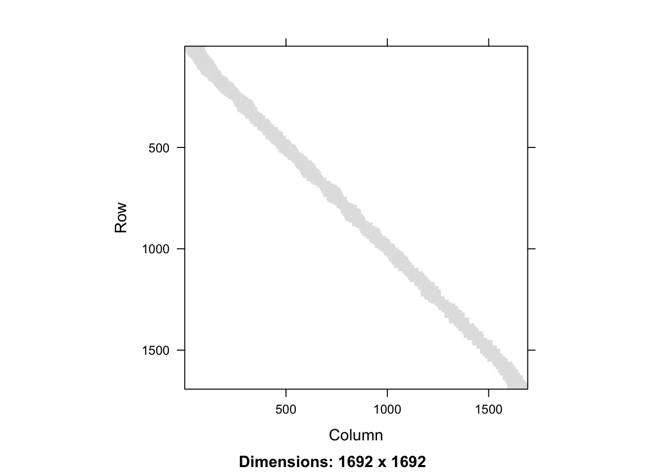
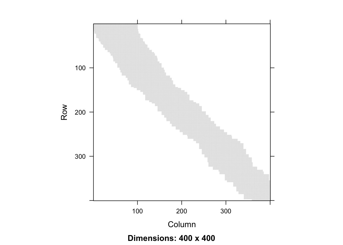
Figure 3.6: Full smoother matrix (left) for \(k\)-nearest neighbor smoothing with \(k = 100\) and the 400 x 400 upper left part (right).

We can then compute the smoother for the greenland temperature data and add it to the scatterplot. Figure 3.7 shows the result. We note that the smoother overall looks quite similar to the kernel smoother in Figure 3.5, though it is somewhat more irregular.

x <- greenland$Temp_Qaqortoq
y <- greenland$Temp_diff
ord <- order(x)
x_ord <- x[ord]
y_ord <- y[ord]
S <- knn_S(x, k = 100)
p_greenland + 
  geom_line(aes(x = x_ord, y = S %*% y_ord), color = "blue", lwd = 1)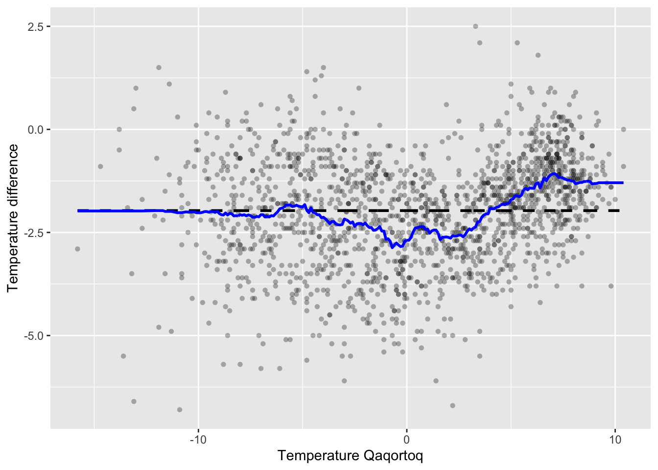

Figure 3.7: The \(k\)-nearest neighbor smoother (blue) with \(k = 100\) added to the greenland temperature scatterplot.

Before we turn to optimization of the tuning parameter \(k\), we will investigate our implementation of the kernel smoother in greater detail. We note, in particular, that the smoother matrix is rather sparse, and computing and storing the full smoother matrix might not be the computationally most efficient solution.

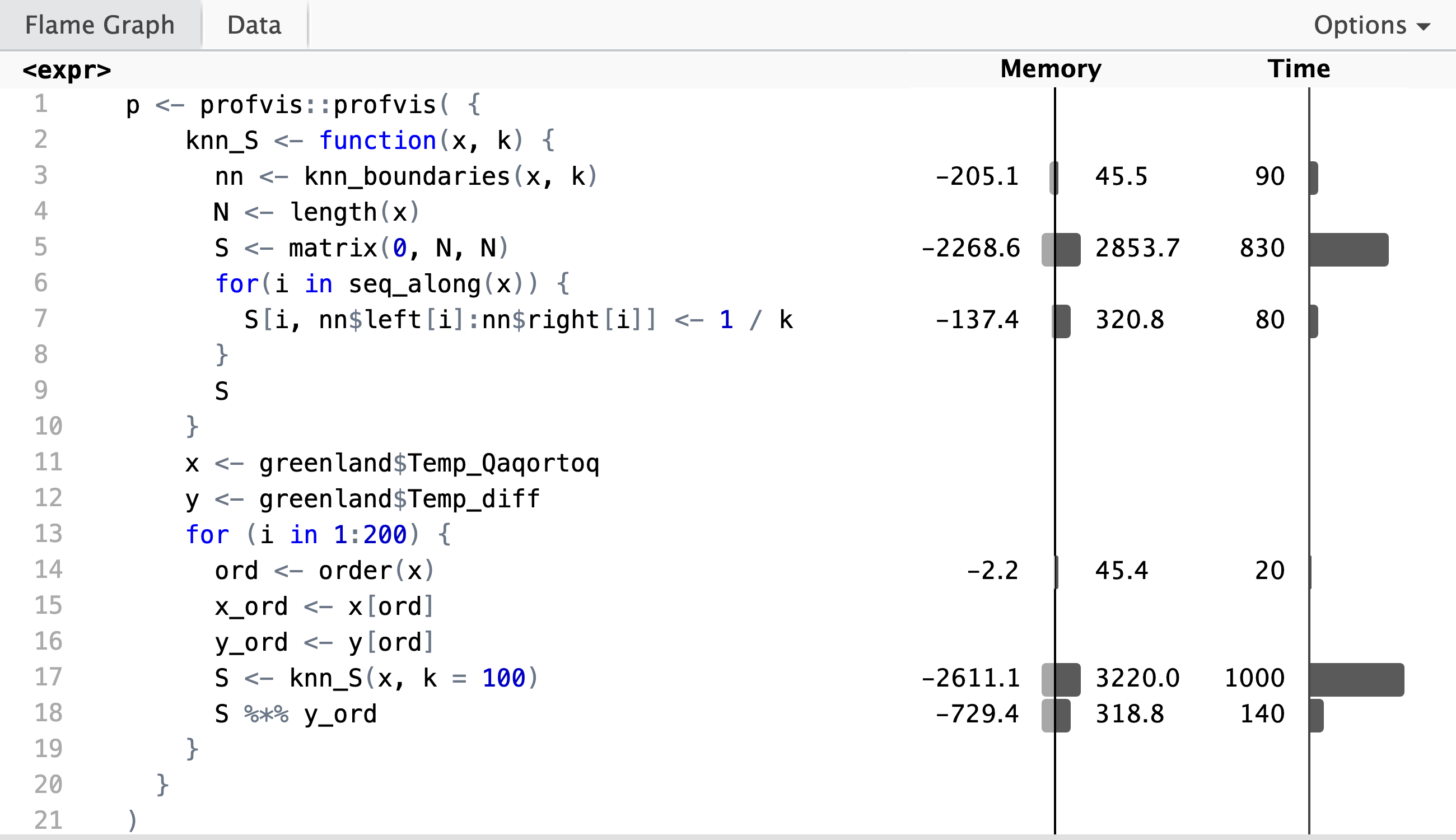
Profiling reveals that it is the construction of the smoother matrix that takes most of the runtime, while the computation of the matrix-vector product, \(\mathbf{S} \mathbf{y}\), in line 19 only takes about 10% of the total runtime. The profiling data shows that the computation of the neighborhood boundaries (line 4) is negligible, and that it is the creation of \(N \times N\) zero-matrix in line 6 that dominates the runtime. Inspection of the flame graph in the interactive HTML widget shows that the real culprit is the garbage collector, which is frequently triggered by the creation of the roughly 23 MB smoother matrix. Runtime is thus primarily spend on allocation and deallocation of memory.

If we revisit (3.4), we see that we can rewrite the mean in terms of the neighborhood boundaries as

\[\begin{equation} \hat{f}_i = \frac{1}{k} \sum_{j = \mathrm{left}_i}^{\mathrm{right}_i} y_j. \tag{3.5} \end{equation}\]

This suggests that we can compute \(k\)-nearest neighbor smoothing without computing \(\mathbf{S}\) but by sequentially computing means over segments of the data vector containing the \(y_i\)-s. This is implemented by the knn_mean() function below.

knn_mean <- function(x, y, k) {
  if (is.unsorted(x)) {
    ord <- order(x)
    x <- x[ord]
    y <- y[ord]
  }
  N <- length(x)
  y_sum <- numeric(N)
  nn <- knn_boundaries(x, k)
  for(i in seq_along(x)) {
      y_sum[i] <- sum(y[nn$left[i]:nn$right[i]])
  }
  data.frame(x = x, y = y_sum / k)
}

knn_greenland <- knn_mean(greenland$Temp_Qaqortoq, greenland$Temp_diff, k = 100)
range(knn_greenland$y - S %*% y_ord)

## [1] -3.109e-15  1.110e-15

knn <- function(x, y, k) {
  if (is.unsorted(x)) {
    ord <- order(x)
    x <- x[ord]
    y <- y[ord]
  }
  N <- length(x)
  y_sum <- numeric(N)
  nn <- knn_boundaries(x, k)
  l <- nn$left[1]
  r <- nn$right[1]
  y_sum[1] <- sum(y[l:r])
  for(i in seq_along(x)[-1]) {
    diff <- 0    
    if (nn$right[i] > r) {
      diff <- sum(y[(r + 1):nn$right[i]] - y[l:(nn$left[i] - 1)])
    }
    y_sum[i] <- y_sum[i - 1] + diff
    l <- nn$left[i]
    r <- nn$right[i]
  }
  data.frame(x = x, y = y_sum / k)
}

knn_greenland <- knn(greenland$Temp_Qaqortoq, greenland$Temp_diff, k = 100)
range(knn_greenland$y - S %*% y_ord)

## [1] -1.332e-15  1.998e-15

bench::mark(
  matrix = c(knn_S(x, k = 100) %*% y_ord),
  knn_mean = knn_mean(x, y, k = 100)$y,
  knn = knn(x, y, k = 100)$y
)

## # A tibble: 3 × 6
##   expression      min   median `itr/sec` mem_alloc `gc/sec`
##   <bch:expr> <bch:tm> <bch:tm>     <dbl> <bch:byt>    <dbl>
## 1 matrix       4.51ms   4.84ms      184.    22.7MB    15.6 
## 2 knn_mean     1.65ms   1.76ms      561.     2.2MB     5.03
## 3 knn        812.17µs    901µs     1109.   148.3KB     2.10

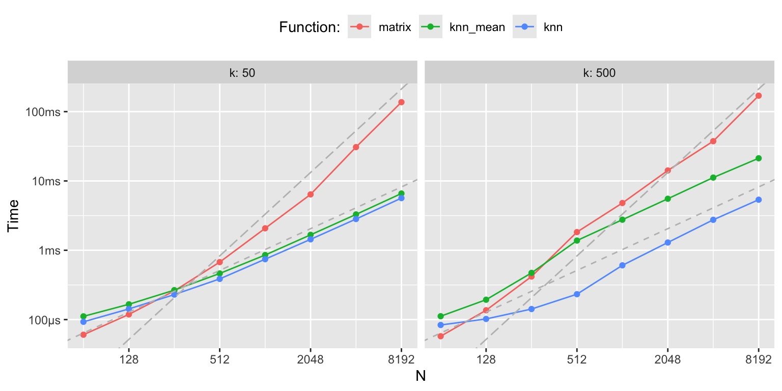
Figure 3.8: k-nearest neighbor benchmarks

loocv_knn <- function(x, y, k) {
  ord <- order(x)
  x <- x[ord]
  y <- y[ord]
  error <- function(k) {
     diag_S <- rep(1/k, length(x))
     f_hat <-  knn(x, y, k)
     loocv_error(f_hat$x, f_hat$y, diag_S)
  }
  sapply(k, error)
}

ks <- seq(50, 1000, 5)
CV <- loocv_knn(greenland$Temp_Qaqortoq, greenland$Temp_diff, ks)
k_opt <- ks[which.min(CV)]
ggplot(mapping = aes(ks, CV)) + geom_point() +
  geom_vline(xintercept = k_opt, color = "red")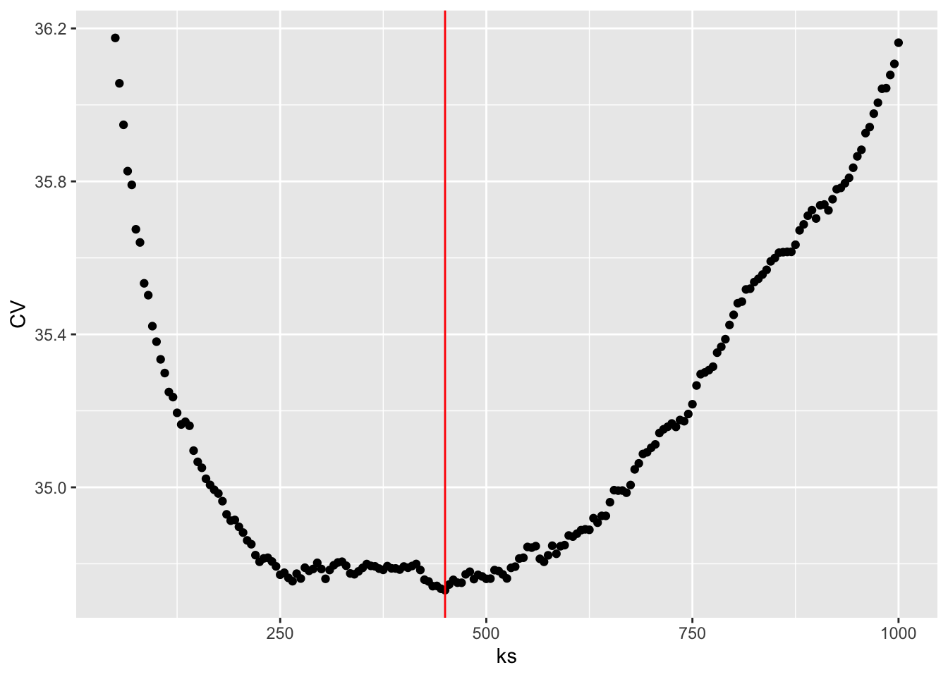

knn_greenland_opt <- knn(
  greenland$Temp_Qaqortoq, 
  greenland$Temp_diff, 
  k = k_opt
)
p_greenland + 
  geom_line(data = knn_greenland_opt, aes(x, y), color = "blue", lwd = 1)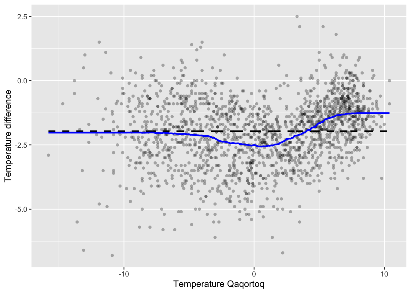

3.5 Polynomial and spline expansions

We return in this section to global models like the linear smoother in Section 3. To make the models flexible, and thus better capable of adapting to local variation in the data, we define the models in terms of basis expansions. That is, we suppose that the function \(f\) can be written as

\[ f = \sum_{i=1}^p \beta_i \varphi_i \]

for basis functions \(\varphi_1, \ldots, \varphi_p : \mathbb{R} \to \mathbb{R}\) and parameters \(\beta_1, \ldots, \beta_p \in \mathbb{R}\).

With \(x_1, \ldots, x_N \in \mathbb{R}\) we define the \(N \times p\) model matrix \(\boldsymbol{\Phi}\) with entries

\[ \Phi_{ij} = \varphi_j(x_i) \]

Letting \(f_i = f(x_i) = (\boldsymbol{\Phi} \beta)_i\) we can write the squared error loss function in terms of \(\mathbf{f}\) as

\[ L(\mathbf{f}) = \sum_{j=1}^N (y_j - f_i)^2 = (\mathbf{y} - \mathbf{f})^T (\mathbf{y} - \mathbf{f})^T = (\mathbf{y} - \boldsymbol{\Phi} \beta)^T (\mathbf{y} - \boldsymbol{\Phi} \beta). \]

The least squares optimizer in terms of \(\beta\) is given as \(\hat{\beta} = (\boldsymbol{\Phi}^T \boldsymbol{\Phi})^{-1} \boldsymbol{\Phi}^T \mathbf{y}\), and in terms of \(\mathbf{f}\) we have

\[ \hat{\mathbf{f}} = \boldsymbol{\Phi} \hat{\beta} = \boldsymbol{\Phi} (\boldsymbol{\Phi}^T \boldsymbol{\Phi})^{-1} \boldsymbol{\Phi}^T \mathbf{y}. \]

The smoother matrix \(\mathbf{S} = \boldsymbol{\Phi} (\boldsymbol{\Phi}^T \boldsymbol{\Phi})^{-1} \boldsymbol{\Phi}^T\) is the orthogonal projection onto the subspace of \(\mathbb{R}^N\) spanned by the columns of \(\boldsymbol{\Phi}\).

In the previous section orthogonality of basis functions played an important role for computing basis function expansions efficiently as well as for the statistical assessment of estimated coefficients. This section will deal with bivariate smoothing via basis functions that are not necessarily orthogonal.

3.5.1 Polynomial expansions

Degree 19 polynomial fitted to the temperature data.

EDIT

We also plot the monthly average temperature, \(Y\), in Nuuk against the the monthly average temperature, \(X\), in Qaqortoq—a town further south of Nuuk in greenland.

Monthly temperature difference between Nuuk and Qaqortoq plottet against the temperature in Qaqortoq. The horizontal dashed line is the average temperature difference, and the straight line smoother (purple) and a spline smoother (blue) are added. Nuuk average monthly temperature against Qaqortoq average monthly temperature smoothed using a straight line (blue) and a smooth spline (red).

In the example shown in Figure 3.2 both the variables are random. We are in this case interested in how the temperature in Qaqortoq is predictive of the temperature in Nuuk.

EDIT

We can extract the model matrix from the lm-object.

N <- nrow(greenland)
intercept <- rep(1/sqrt(N), N)  # To make intercept column have norm one
polylm <- lm(Temp_diff ~ intercept + poly(Temp_Qaqortoq, 15) - 1, data = greenland)
Phi <- model.matrix(polylm)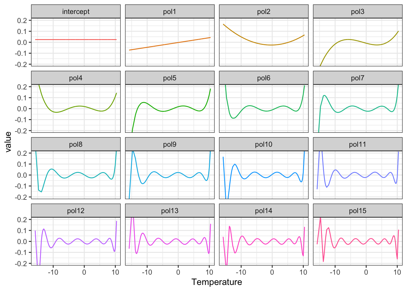

Figure 3.9: The model matrix columns as functions

The model matrix is (almost) orthogonal, and estimation becomes quite simple. With an orthogonal model matrix the normal equation reduces to the estimate

\[ \hat{\beta} = \Phi^T Y \]

since \(\Phi^T \Phi = I\). The predicted (or fitted) values are \(\Phi \Phi^T Y\) with smoother matrix \(\mathbf{S} = \Phi \Phi^T\) being a projection.

(t(Phi) %*% greenland$Temp_diff)[1:10, 1]

##                intercept poly(Temp_Qaqortoq, 15)1 poly(Temp_Qaqortoq, 15)2 
##                 -81.0426                  10.4477                  13.3838 
## poly(Temp_Qaqortoq, 15)3 poly(Temp_Qaqortoq, 15)4 poly(Temp_Qaqortoq, 15)5 
##                   5.2623                  -4.6766                  -6.3974 
## poly(Temp_Qaqortoq, 15)6 poly(Temp_Qaqortoq, 15)7 poly(Temp_Qaqortoq, 15)8 
##                  -1.3931                   3.5555                   1.7287 
## poly(Temp_Qaqortoq, 15)9 
##                   0.5038

coef(polylm)[1:10]

##                intercept poly(Temp_Qaqortoq, 15)1 poly(Temp_Qaqortoq, 15)2 
##                 -81.0426                  10.4477                  13.3838 
## poly(Temp_Qaqortoq, 15)3 poly(Temp_Qaqortoq, 15)4 poly(Temp_Qaqortoq, 15)5 
##                   5.2623                  -4.6766                  -6.3974 
## poly(Temp_Qaqortoq, 15)6 poly(Temp_Qaqortoq, 15)7 poly(Temp_Qaqortoq, 15)8 
##                  -1.3931                   3.5555                   1.7287 
## poly(Temp_Qaqortoq, 15)9 
##                   0.5038

With homogeneous variance

\[ \hat{\beta}_i \overset{\text{approx}}{\sim} \mathcal{N}(\beta_i, \sigma^2), \]

and for \(\beta_i = 0\) we have \(P(|\hat{\beta}_i| \geq 1.96\sigma) \approx 0.05.\)

Thresholding:

## Warning: Using `size` aesthetic for lines was deprecated in ggplot2 3.4.0.
## ℹ Please use `linewidth` instead.
## This warning is displayed once every 8 hours.
## Call `lifecycle::last_lifecycle_warnings()` to see where this warning was
## generated.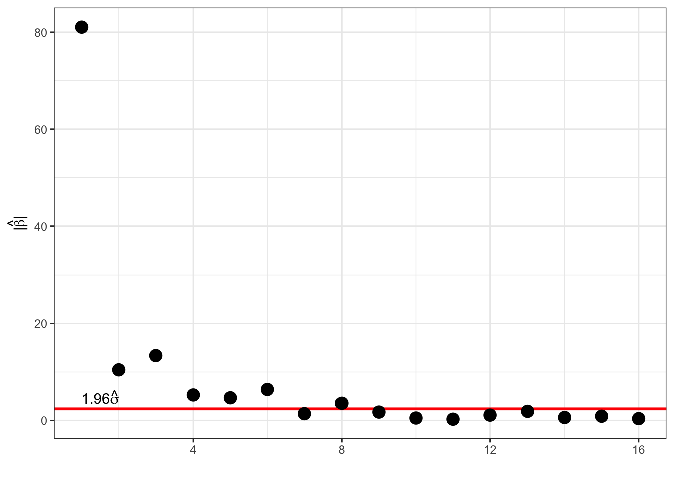

factor <- 1.96
selected_coef <- which(abs(coef(polylm)) > factor * sigmahat)
f_hat <- Phi[, selected_coef] %*% coef(polylm)[selected_coef]
p_greenland + 
  geom_smooth(
    method = "lm",
    formula = y ~ poly(x, 15),       # A polynomial smoother
    se = FALSE,
    color = "red"
  ) +
  geom_line(aes(y = f_hat), color = "blue", lwd = 1)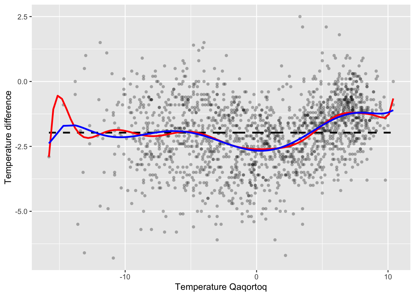

3.5.2 Smoothing splines

To motivate splines we briefly consider the following penalized least squares criterion for finding a smooth approximation to bivariate data: minimize

\[\begin{equation} L(f) = \sum_{i=1}^N (y_i - f(x_i))^2 + \lambda \|f''\|_2^2 \tag{3.6} \end{equation}\]

over all twice differentiable functions \(f\). The first term is the standard squared error, and we can easily find a smooth function interpolating the \(y\)-values (if all the \(x\)-values are different), which will thus drive the squared error to 0. The squared 2-norm regularizes the minimization problem so that the minimizer finds a balance between interpolation and having a small second derivative (note that \(\|f''\|_2 = 0\) if and only if \(f\) is an affine function). The tuning parameter \(\lambda\) controls this balance.

It is possible to show that the minimizer of (3.6) is a natural cubic spline with knots in the data points \(x_i\). That is, the spline is a \(C^2\)-function that equals a third degree polynomial in between the knots. At the knots, the two polynomials that meet fit together up to the second derivative, but they may differ on the third derivative. That the solution is natural means that it has zero second and third derivative at and beyond the two boundary knots.

It is not particularly difficult to show that the space of natural cubic splines is a vector space of dimension \(N\) if all the \(x\)-values are different. It is therefore possible to find a basis of splines, \(\varphi_1, \ldots, \varphi_N\), such that the \(f\) that minimizes (3.6) is of the form

\[ f = \sum_{i=1}^N \beta_i \varphi_i. \]

What is remarkable about this is that the basis (and the finite dimensional vector space it spans) does not depend upon the \(y\)-values. Though the optimization is over an infinite dimensional space, the penalization ensures that the minimizer is always in the same finite dimensional space nomatter what \(y_1, \ldots, y_N\) are. Moreover, since (3.6) is a quite natural criterion to minimize to find a smooth function fitting the bivariate data, splines appear as good candidates for producing such smooth fits. On top of that, splines have several computational advantages and are widely used.

If we let \(\hat{f}_i = \hat{f}(x_i)\) with \(\hat{f}\) the minimizer of (3.6), we have in vector notation that

\[ \hat{\mathbf{f}} = \boldsymbol{\Phi}\hat{\beta} \]

with \(\boldsymbol{\Phi}_{ij} = \varphi_j(x_i)\). The minimizer can be found by observing that

\[\begin{align} L(\mathbf{f}) & = (\mathbf{y} - \mathbf{f})^T (\mathbf{y} - \mathbf{f}) + \lambda \| f'' \|_2^2 \\ & = ( \mathbf{y} - \boldsymbol{\Phi}\beta)^T (\mathbf{y} - \boldsymbol{\Phi}\beta) + \lambda \beta^T \boldsymbol{\Omega} \beta \end{align}\]

where

\[ \boldsymbol{\Omega}_{ij} = \langle \varphi_i'', \varphi_j'' \rangle = \int \varphi_i''(z) \varphi_j''(z) \mathrm{d}z. \]

The matrix \(\boldsymbol{\Omega}\) is positive semidefinite by construction, and we refer to it as the penalty matrix. It induces a seminorm on \(\mathbb{R}^N\) so that we can express the seminorm, \(\|f''\|_2\), of \(f\) in terms of the parameters in the basis expansion using \(\varphi_i.\)

Minimizing \(L(\mathbf{f})\) is a standard penalized least squares problem, whose solution in terms of the \(\beta\)-parameter is

\[ \hat{\beta} = (\boldsymbol{\Phi}^T \boldsymbol{\Phi} + \lambda \boldsymbol{\Omega})^{-1}\boldsymbol{\Phi}^T \mathbf{y} \]

and with resulting smoother

\[ \hat{\mathbf{f}} = \underbrace{\boldsymbol{\Phi} ((\boldsymbol{\Phi}^T \boldsymbol{\Phi} + \lambda \boldsymbol{\Omega})^{-1}\boldsymbol{\Phi}^T}_{\mathbf{S}_{\lambda}} \mathbf{y}. \]

This linear smoother with smoothing matrix \(\mathbf{S}_{\lambda}\) based on natural cubic splines gives what is known as a smoothing spline that minimizes (3.6).

We will pursue spline based smoothing by minimizing (3.6) but using various B-spline bases that may have more or less than \(N\) elements. For the linear algebra, it actually does not matter if we use a spline basis or any other basis—as long as \(\boldsymbol{\Phi}_{ij} = \varphi_j(x_i)\) and \(\boldsymbol{\Omega}\) is given in terms of \(\varphi''_i\) as above.

3.5.3 Splines in R

Though some of the material of this section will apply to any choice of basis, we restrict attention to splines and consider almost exclusively the widely used B-splines (the “B” is for basis).

The splines package in R implements some of the basic functions needed to work with splines. In particular, the splineDesign() function that computes evaluations of B-splines and their derivatives.

library(splines)

# Note the specification of repeated boundary knots
knots <- c(0, 0, 0, seq(0, 1, 0.2), 1, 1, 1)
xx <- seq(0, 1, 0.005)
B_splines <- splineDesign(knots, xx)
matplot(xx, B_splines, type = "l", lty = 1)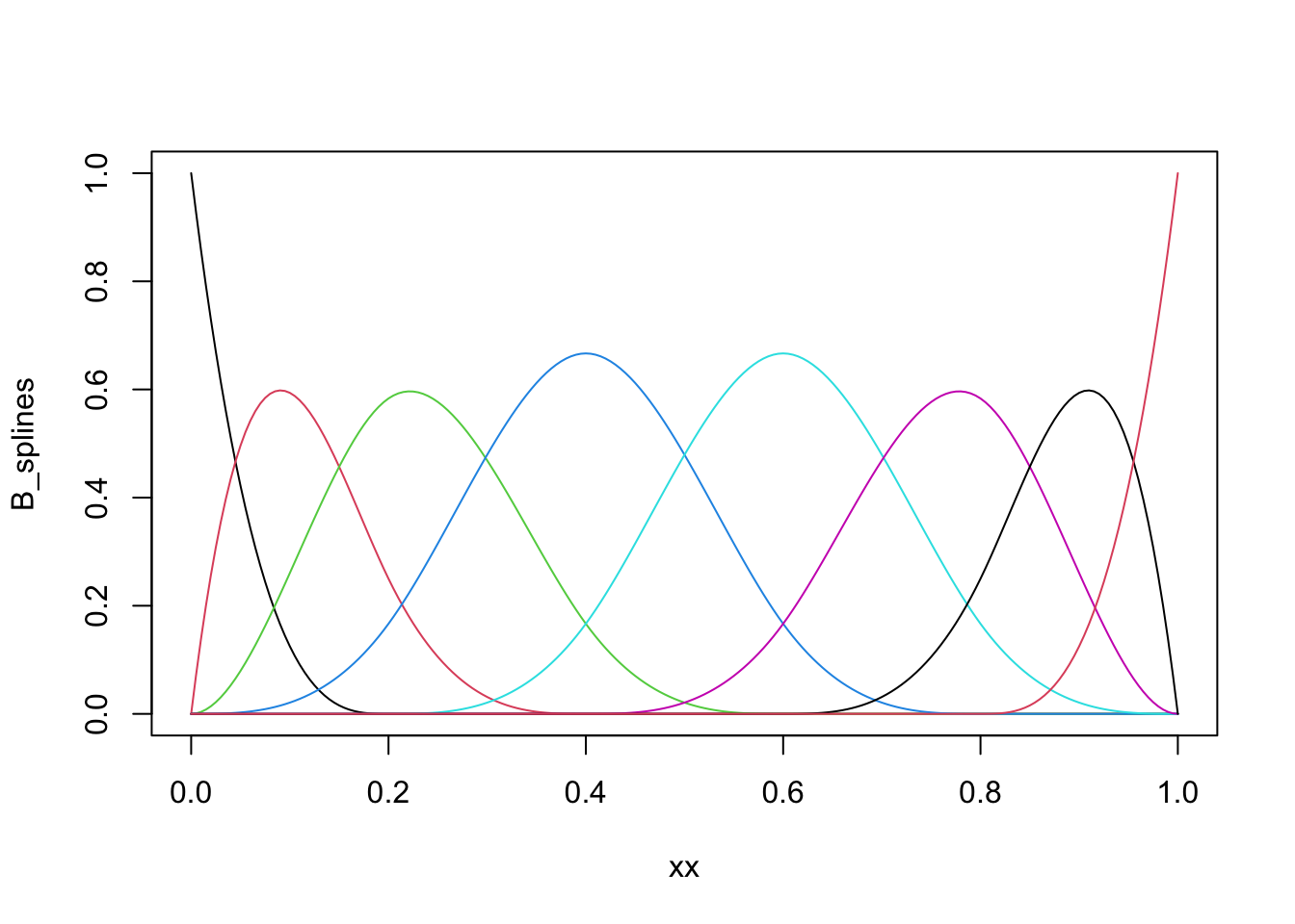

Figure 3.10: B-spline basis as computed by `splineDesign().

The basis shown in Figure 3.10 is an example of a cubic B-spline basis with the 11 inner knots \(0, 0.1, \ldots, 0.9, 1\). The repeated boundary knots control how the spline basis behaves close to the boundaries of the interval. This basis has 13 basis functions, not 11, and spans a larger space than the space of natural cubic splines. It is possible to compute a basis based on B-splines for the natural cubic splines using the function ns, but for all practical purposes this is not important, and we will work exclusively with the B-spline basis itself.

The computation of the penalty matrix \(\boldsymbol{\Omega}\) constitutes a practical problem, but observing that \(\varphi''_i\) is an affine function in between knots leads to a simple way of computing \(\boldsymbol{\Omega}_{ij}\). Letting \(g_{ij} = \varphi''_i \varphi''_j\) it holds that \(g_{ij}\) is quadratic between two consecutive knots \(a\) and \(b\), in which case

\[ \int_a^b g_{ij}(z) \mathrm{d}z = \frac{b - a}{6}\left(g_{ij}(a) + 4 g_{ij}\left(\frac{a + b}{2}\right) + g_{ij}(b)\right). \]

This identity is behind Simpson’s rule for numerical integration, and the fact that this is an identity for quadratic polynomials, and not an approximation, means that Simpson’s rule applied appropriately leads to exact computation of \(\boldsymbol{\Omega}_{ij}\). All we need is the ability to evaluate \(\varphi''_i\) at certain points, and splineDesign() can be used for that.

pen_mat <- function(inner_knots) {
  knots <- sort(c(rep(range(inner_knots), 3), inner_knots))
  d <- diff(inner_knots)  # The vector of knot differences; b - a 
  g_ab <- splineDesign(knots, inner_knots, derivs = 2) 
  knots_mid <- inner_knots[-length(inner_knots)] + d / 2
  g_ab_mid <- splineDesign(knots, knots_mid, derivs = 2)
  g_a <- g_ab[-nrow(g_ab), ]
  g_b <- g_ab[-1, ]
  (crossprod(d * g_a,  g_a) + 
      4 * crossprod(d * g_ab_mid, g_ab_mid) + 
      crossprod(d * g_b, g_b)) / 6 
}

It is laborious to write good tests of pen_mat(). We would have to work out a set of example matrices by other means, e.g. by hand. Alternatively, we can compare to a simpler numerical integration technique using Riemann sums.

spline_deriv <- splineDesign(
  c(0, 0, 0, 0, 0.5, 1, 1, 1, 1), 
  seq(0, 1, 1e-5), 
  derivs = 2
)
Omega_numeric <- crossprod(spline_deriv[-1, ]) * 1e-5  # Right Riemann sums
Omega <- pen_mat(c(0, 0.5, 1))
Omega_numeric / Omega

##        [,1] [,2]   [,3] [,4] [,5]
## [1,] 1.0000    1 0.9999    1  NaN
## [2,] 1.0000    1 1.0000    1    1
## [3,] 0.9999    1 1.0000    1    1
## [4,] 1.0000    1 1.0000    1    1
## [5,]    NaN    1 1.0001    1    1

range((Omega_numeric - Omega) / (Omega + 0.001))  #  Relative error

## [1] -6e-05  6e-05

And we should also test an example with non-equidistant knots.

spline_deriv <- splineDesign(
  c(0, 0, 0, 0, 0.2, 0.3, 0.5, 0.6, 0.65, 0.7, 1, 1, 1, 1), 
  seq(0, 1, 1e-5), 
  derivs = 2
)
Omega_numeric <- crossprod(spline_deriv[-1, ]) * 1e-5  # Right Riemann sums
Omega <- pen_mat(c(0, 0.2, 0.3, 0.5, 0.6, 0.65, 0.7, 1))
range((Omega_numeric - Omega) / (Omega + 0.001)) # Relative error

## [1] -0.0001607  0.0002545

These examples indicate that pen_mat() computes \(\boldsymbol{\Omega}\) correctly, in particular as increasing the Riemann sum precision by lowering the number \(10^{-5}\) will decrease the relative error (not shown). Of course, correctness ultimately depends on splineDesign() computing the correct second derivatives, which hasn’t been tested here.

We can also test how our implementation of smoothing splines works on data. We do this here by implementing the matrix-algebra directly for computing \(\mathbf{S}_{\lambda} \mathbf{y}\).

ord <- order(greenland$Temp_Qaqortoq)
x <- greenland$Temp_Qaqortoq[ord]
y <- greenland$Temp_diff[ord]
inner_knots <- unique(x)
Phi <- splineDesign(c(rep(range(inner_knots), 3), inner_knots), x)
Omega <- pen_mat(inner_knots)
smoother <- function(lambda) 
  Phi %*% solve(
    crossprod(Phi) + lambda * Omega, 
    t(Phi) %*% y
  )
p_greenland + 
  geom_line(aes(x = x, y = smoother(0.1)), color = "red", linewidth = 1) +      # Undersmooth
  geom_line(aes(x = x, y = smoother(100)), color = "blue", linewidth = 1) +     # Smooth
  geom_line(aes(x = x, y = smoother(100000)), color = "purple", linewidth = 1)  # Oversmooth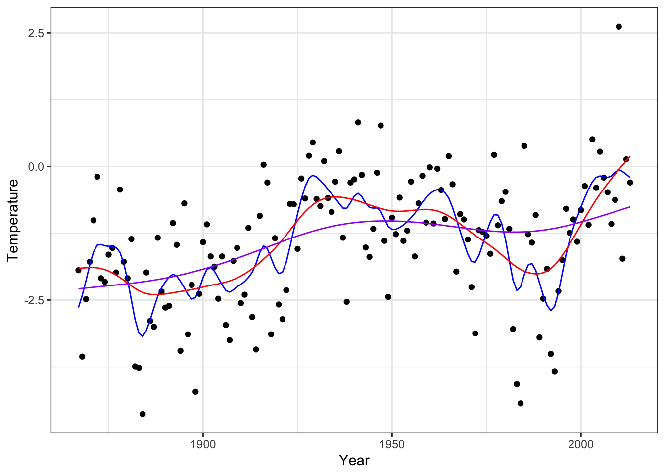

Smoothing splines can be computed using the R function smooth.spline() from the stats package. It is possible to manually specify the amount of smoothing using one of the arguments lambda, spar or df (the latter being the trace of the smoother matrix). However, due to internal differences from the splineDesign() basis above, the lambda argument to smooth.spline() does not match the \(\lambda\) parameter above.

If the amount of smoothing is not manually set, smooth.spline() chooses \(\lambda\) by generalized cross validation (GCV), which minimizes

\[ \mathrm{GCV} = \sum_{i=1}^N \left(\frac{y_i - \hat{f}_i}{1 - \mathrm{df} / n}\right)^2, \]

where

\[ \mathrm{df} = \mathrm{trace}(\mathbf{S}) = \sum_{i=1}^N S_{ii}. \]

GCV corresponds to LOOCV with the diagonal entries, \(S_{ii}\), replaced by their average \(\mathrm{df} / n\). The main reason for using GCV over LOOCV is that for some smoothers, such as the spline smoother, it is possible to compute the trace \(\mathrm{df}\) easily without computing \(\mathbf{S}\) or even its diagonal elements.

To compare our results to smooth.spline() we optimize the GCV criterion. First we implement a function that computes GCV for a fixed value of \(\lambda\). Here the implementation is relying on computing the smoother matrix, but this is not the most efficient implementation. Section 3.5.4 provides a diagonalization of the smoother matrix jointly in the tuning parameters. This representation allows for efficient computation with splines, and it will become clear why it is not necessary to compute \(\mathbf{S}\) or even its diagonal elements. The trace is nevertheless easily computable \(\mathbf{S}\).

gcv <- function(lambda, y) {
  S <- Phi %*% solve(crossprod(Phi) + lambda * Omega, t(Phi))
  df <- sum(diag(S))  # The trace of the smoother matrix
  sum(((y - S %*% y) / (1 - df / length(y)))^2, na.rm = TRUE) 
}

Then we apply this function to a grid of \(\lambda\)-values and choose the value of \(\lambda\) that minimizes GCV.

lambda <- seq(50, 250, 2)
GCV <- sapply(lambda, gcv, y = y)
lambda_opt <- lambda[which.min(GCV)]
ggplot(mapping = aes(lambda, GCV)) + geom_point() +
  geom_vline(xintercept = lambda_opt, color = "red")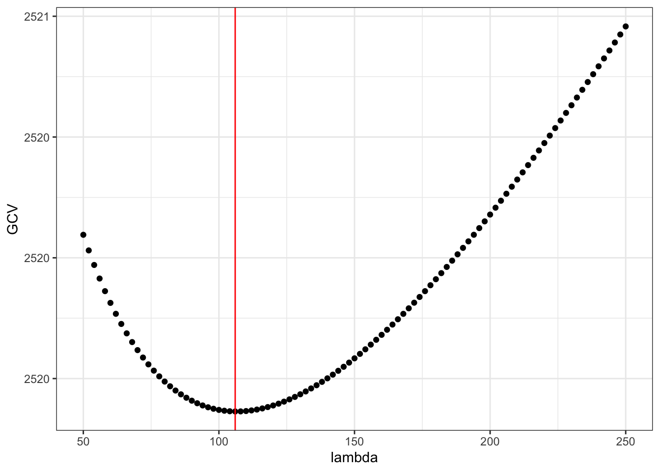

Figure 3.11: The generalized cross-validation criterion for smoothing splines as a function of the tuning parameter \(\lambda\).

Finally, we can visualize the resulting smoothing spline.

smooth_opt <- Phi %*% solve(
  crossprod(Phi) + lambda_opt * Omega, 
  t(Phi) %*% y
)
p_greenland + 
  geom_line(aes(x = x, y = smooth_opt), color = "blue", lwd = 1)

Figure 3.12: The smoothing spline that minimizes GCV over the tuning parameter \(\lambda\)

The smoothing spline that we found by minimizing GCV can be compared to the smoothing spline that smooth.spline() computes by minimizing GCV as well.

smooth_splines <- smooth.spline(
  greenland$Temp_Qaqortoq, 
  greenland$Temp_diff, 
  all.knots = TRUE        # Don't use heuristic
)  
range(smooth_splines$y - smooth_opt[!duplicated(x)])

## [1] -0.0001726  0.0005263

p_greenland + 
  geom_line(data = data.frame(x = smooth_splines$x, y = smooth_splines$y), 
    aes(x, y), color = "blue", lwd = 1)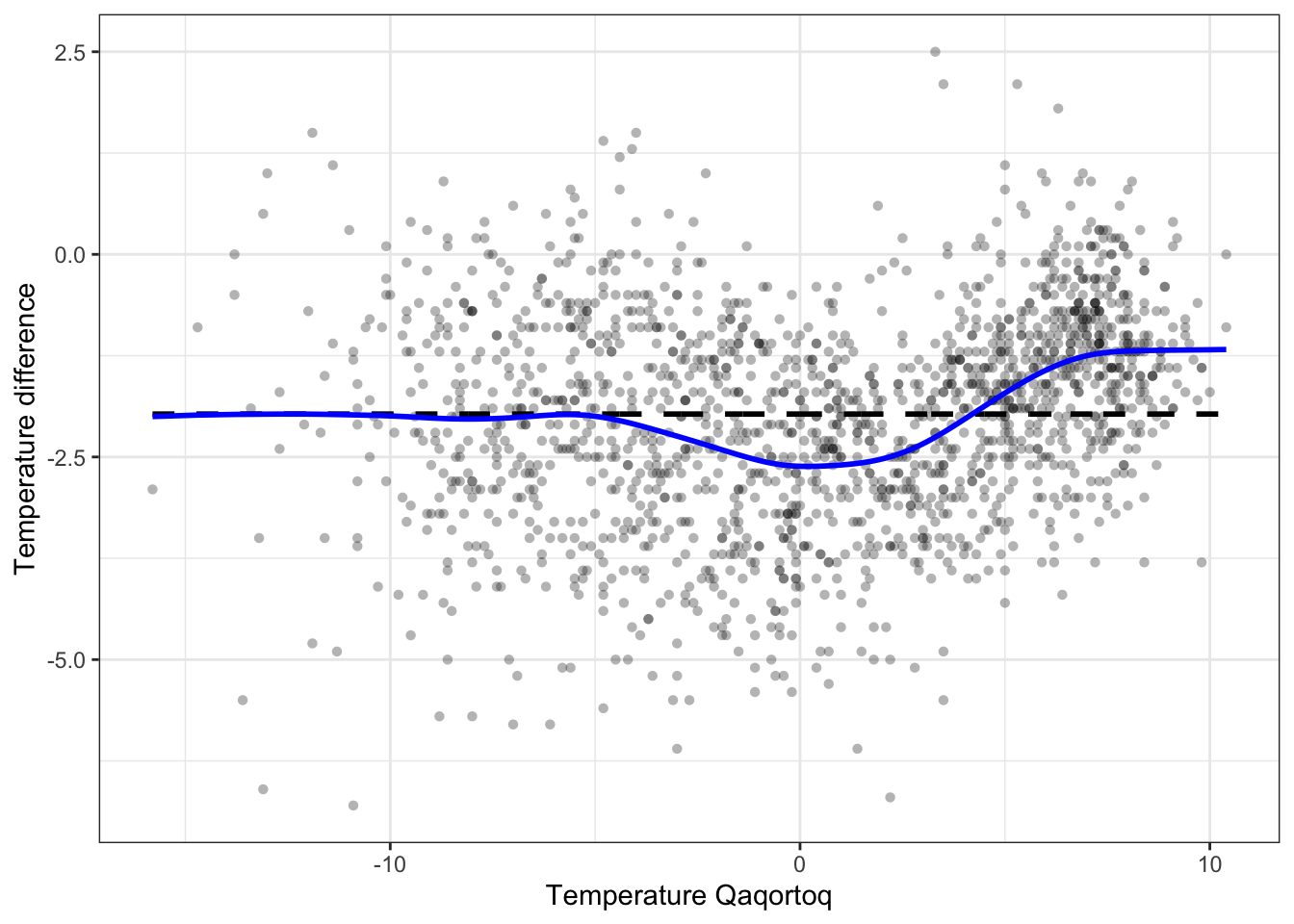

Figure 3.13: The smoothing spline that minimizes GCV as computed by smooth.spline().

The differences between the smoothing spline computed by our implementation and by smooth.spline() is hardly detectable visually, and they are at most of the order \(10^{-3}\) as computed above. It is possible to further decrease the differences by finding the optimal value of \(\lambda\) with a higher precision, but we will not pursue this here.

3.5.4 Efficient computation with splines

Using the full B-spline basis with knots in every observation is computationally heavy and from a practical viewpoint unnecessary. Smoothing using B-splines is therefore often done using a knot-selection heuristic that selects much fewer knots than \(n\), in particular if \(n\) is large. This is also what smooth.spline() does unless all.knots = TRUE. The heuristic for selecting the number of knots is a bit complicated, but it is implemented in the function .nknots.smspl(), which can be inspected for details. Once the number of knots gets above 200 it grows extremely slowly with \(n\). With the number of knots selected, a common heuristic for selecting their position is to use the quantiles of the distribution of the \(x\)-values. That is, with 9 knots, say, the knots are positioned in the deciles (0.1-quantile, 0.2-quantile etc.). This is effectively also what smooth.spline() does, and this heuristic places most of the knots where we have most of the data points.

Having implemented a knot-selection heuristic that results in \(p\) B-spline basis functions, the matrix \(\Phi\) will be \(N \times p\), typically with \(p < N\) and with \(\Phi\) of full rank \(p\). In this case we derive a way of computing the smoothing spline that is computationally more efficient and numerically more stable than relying on the matrix-algebraic solution above. This is particularly so when we need to compute the smoother for many different \(\lambda\)-s to optimize the smoother. As we will show, we are effectively computing a simultaneous diagonalization of the (symmetric) smoother matrix \(\mathbf{S}_{\lambda}\) for all values of \(\lambda\).

The matrix \(\Phi\) has a singular value decomposition

\[ \Phi = \mathbf{U} D \mathbf{V}^T \]

where \(D\) is diagonal with entries \(d_1 \geq d_2 \geq \ldots \geq d_p > 0\), \(\mathbf{U}\) is \(n \times p\), \(\mathbf{V}\) is \(p \times p\) and both are orthogonal matrices. This means that

\[ \mathbf{U}^T \mathbf{U} = \mathbf{V}^T \mathbf{V} = \mathbf{V} \mathbf{V}^T = I \]

is the \(p \times p\) dimensional identity matrix. We find that

\[\begin{align} \mathbf{S}_{\lambda} & = \mathbf{U}D\mathbf{V}^T(\mathbf{V}D^2\mathbf{V}^T + \lambda \boldsymbol{\Omega})^{-1} \mathbf{V}D\mathbf{U}^T \\ & = \mathbf{U}D (D^2 + \lambda \mathbf{V}^T \boldsymbol{\Omega} \mathbf{V})^{-1} D \mathbf{U}^T \\ & = \mathbf{U} (I + \lambda D^{-1} \mathbf{V}^T \boldsymbol{\Omega} \mathbf{V} D^{-1})^{-1} \mathbf{U}^T \\ & = \mathbf{U}(I + \lambda \widetilde{\boldsymbol{\Omega}})^{-1} \mathbf{U}^T, \end{align}\]

where \(\widetilde{\boldsymbol{\Omega}} = D^{-1} \mathbf{V}^T \boldsymbol{\Omega} \mathbf{V} D^{-1}\) is a positive semidefinite \(p \times p\) matrix. By diagonalization,

\[ \widetilde{\boldsymbol{\Omega}} = \mathbf{W} \Gamma \mathbf{W}^T, \]

where \(\mathbf{W}\) is orthogonal and \(\Gamma\) is a diagonal matrix with nonnegative values in the diagonal, and we find that

\[\begin{align} \mathbf{S}_{\lambda} & = \mathbf{U} \mathbf{W} (I + \lambda \Gamma)^{-1} \mathbf{W}^T \mathbf{U}^T \\ & = \widetilde{\mathbf{U}} (I + \lambda \Gamma)^{-1} \widetilde{\mathbf{U}}^T \end{align}\]

where \(\widetilde{\mathbf{U}} = \mathbf{U} \mathbf{W}\) is an orthogonal \(n \times p\) matrix.

The interpretation of this representation is as follows.

• First, the coefficients, \(\hat{\beta} = \widetilde{\mathbf{U}}^Ty\), are computed for expanding \(y\) in the basis given by the columns of \(\widetilde{\mathbf{U}}\).
• Second, the \(i\)-th coefficient is shrunk towards 0,

\[ \hat{\beta}_i(\lambda) = \frac{\hat{\beta}_i}{1 + \lambda \gamma_i}. \]

• Third, the smoothed values, \(\widetilde{\mathbf{U}} \hat{\beta}(\lambda)\), are computed as an expansion using the shrunken coefficients.

Thus the smoother works by shrinking the coefficients toward zero in the orthonormal basis given by the columns of \(\widetilde{\mathbf{U}}\). The coefficients corresponding to the largest eigenvalues \(\gamma_i\) are shrunk relatively more toward zero than those corresponding to the small eigenvalues. The basis formed by the columns of \(\widetilde{\mathbf{U}}\) is known as the Demmler-Reinsch basis with reference to (Demmler and Reinsch 1975).

We implement the computation of the diagonalization for the Nuuk temperature data using \(p = 20\) basis functions (18 inner knots) equidistantly distributed over the range of the years for which we have data.

inner_knots <- seq(-15.8, 10.4, length.out = 18)
ord <- order(greenland$Temp_Qaqortoq)
x <- unique(greenland$Temp_Qaqortoq[ord])
Phi <- splineDesign(c(rep(range(inner_knots), 3), inner_knots), x)
Omega <- pen_mat(inner_knots)
Phi_svd <- svd(Phi)
Omega_tilde <- t(crossprod(Phi_svd$v, Omega %*% Phi_svd$v)) / Phi_svd$d
Omega_tilde <- t(Omega_tilde) / Phi_svd$d
# It is safer to use the numerical singular value decomposition ('svd()')
# for diagonalizing a positive semidefinite matrix than to use a 
# more general numerical diagonalization implementation such as 'eigen()'. 
Omega_tilde_svd <- svd(Omega_tilde)  
U_tilde <- Phi_svd$u %*% Omega_tilde_svd$u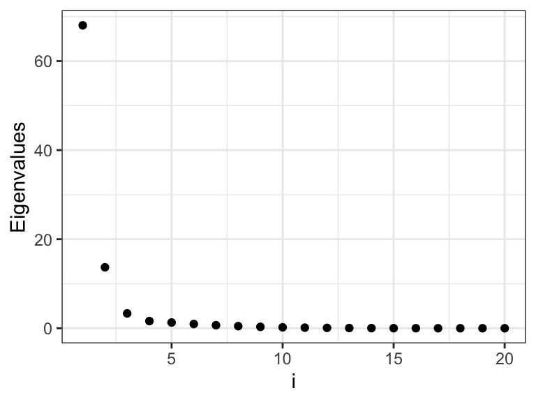

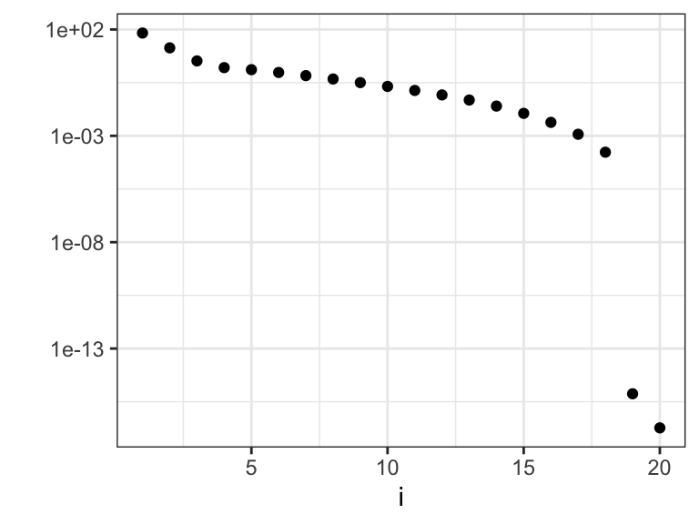
Figure 3.14: The eigenvalues \(\gamma_i\) that determine how much the different basis coefficients in the orthonormal spline expansion are shrunk toward zero. Left plot shows the eigenvalues, and the right plot shows the eigenvalues on a log-scale.

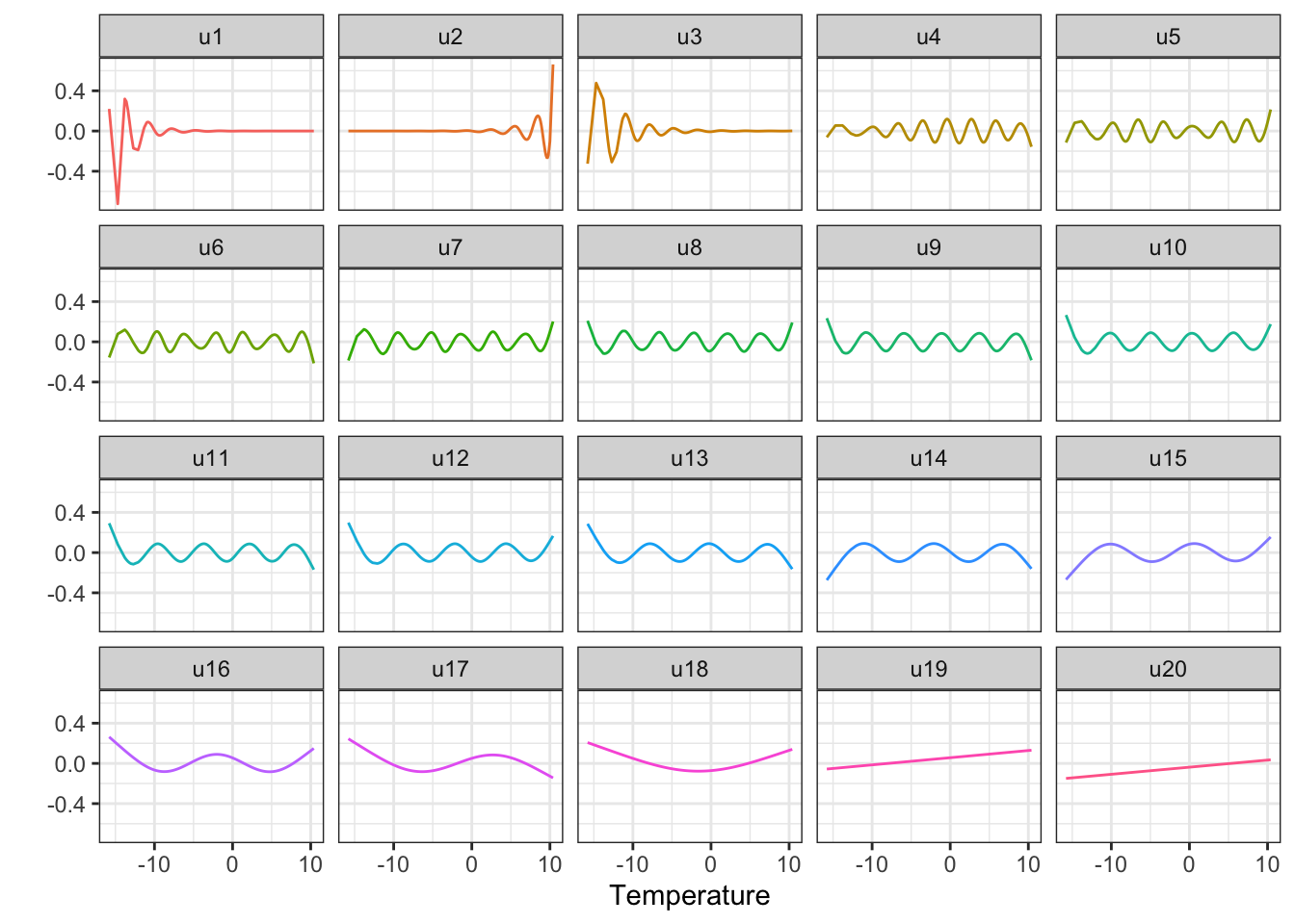
Figure 3.15: The columns of \(\widetilde{\mathbf{U}}\) that consitute an orthonormal basis known as the Demmler-Reinsch basis for computing the spline based smoother.

We observe from Figures 3.14 and 3.15 that there are two relatively large eigenvalues corresponding to the two basis functions with erratic behavior close to the boundaries, and there are two eigenvalues that are effectively zero corresponding to the two affine basis functions. In addition, the more oscillating the basis function is, the larger is the corresponding eigenvalue, and the more is the corresponding coefficient shrunk toward zero by the spline smoother.

Observe also that

\[ \mathrm{df}(\lambda) = \mathrm{trace}(\mathbf{S}_\lambda) = \sum_{i=1}^p \frac{1}{1 + \lambda \gamma_i}, \]

which makes it possible to implement GCV without even computing the diagonal entries of \(\mathbf{S}_{\lambda}.\)

3.6 Exercises

Nearest neighbors

Sparse matrices

Kernel estimators

Exercise 3.1 Consider a bivariate dataset \((x_1, y_1), \ldots, (x_N, y_N)\) and let \(K\) be a probability density with mean 0. Then

\[ \hat{f}(x, y) = \frac{1}{N h^2} \sum_{i=1}^N K\left(\frac{x - x_i}{h}\right) K\left(\frac{y - y_i}{h}\right) \]

is a bivariate kernel density estimator of the joint density of \(x\) and \(y\). Show that the kernel density estimator

\[ \hat{f}_1(x) = \frac{1}{N h} \sum_{i=1}^N K\left(\frac{x - x_i}{h}\right) \] is also the marginal distribution of \(x\) under \(\hat{f}\), and that the Nadaraya-Watson kernel smoother is the conditional expectation of \(y\) given \(x\) under \(\hat{f}\).

Exercise 3.2 Suppose that \(K\) is a symmetric kernel and the \(x\)-s are equidistant. Implement a function that computes the smoother matrix using the toeplitz() function and \(O(n)\) kernel evaluations where \(n\) is the number of data points. Implement also a function that computes the diagonal elements of the smoother matrix directly with runtime \(O(n)\). Hint: find inspiration in the implementation of the running mean.

Exercise 3.3 Use the Gaussian kernel with bandwidth parameter \(h\). Implement the marginal log-likelihood for Gaussian processes as a function of \(h\) and \(\sigma^2\). Using the greenland data and maximise \(\ell\) as a function of \(h\) and \(\sigma^2\) over a grid. Compare the resulting Gaussian process smoother with the optimal Nadaraya–Watson kernel smoother in Figure @(fig:greenland-NN-opt).

Exercise 3.4 Consider the following two functions, k_smallest() and knn_S_outer(). Explain how knn_S_outer() implements the computation of the smoother matrix for \(k\)-nearest neighbors.

k_smallest <- function(x, k) {
  xk <- sort(x, partial = k)[k]
  which(x <= xk)
}

knn_S_outer <- function(x, k) {
  D <- outer(x, x, function(x1, x2) abs(x2 - x1))
  N <- length(x)
  S <- matrix(0, N, N)
  for(i in 1:N) {
    k_indices <- k_smallest(D[i, ], k)[1:k]
    S[i, k_indices] <- 1 / k
  }
  S
}

Compare the implementation with knn_S(). Using the greenland data, explain any differences between the smoother matrix computed using either function.