A R programming
This appendix on R programming is a brief overview of important programming constructs and concepts in R that are used in the book. For a more extensive coverage of R as a programming language, the reader is referred to the book Advanced R (Wickham 2019).
Depending on your background, the appendix can serve different purposes. If you already have experience with programming in R, this appendix can serve as a brush up on some basic aspects of the R language that are used throughout the book. If you have experience with programming in other languages than R, it can serve as an introduction to typical R programming techniques, where some may differ from what you know from other languages. If you have little prior experience with programming, this appendix can teach you the most important things for getting started with the book, but you are encouraged to follow up with additional and more detailed material like the book Advanced R.
Irrespective of your background, this appendix covers topics of greatest relevance for understanding how to implement correct and efficient numerical algorithms used in statistics. These topics are
- data types, comparisons, and numerical precision
- functions and vectorized computations
- environments and function factories
- performance assessment and improvement
- S3 objects and methods
Several other topics of importance for R programming more broadly, such as S4 and R6 objects, expressions, and data wrangling, are not used much in the book and are not covered in any detail in this appendix. The reader is referred to the book R for Data Science (2e) (Wickham et al. 2023) for the use of R and Tidyverse as a framework for handling and visualizing data.
The book will not delve into questions regarding coding style either, but all code presented adheres to the tidyverse style guide unless there are specific reasons to deviate from it. The reader is encouraged to adopt this style guide for their own code, or at least to make conscious and consistent decisions regarding any deviations.
A.1 Data structures
The fundamental data structure in R is a vector. Even variables that look and behave like single numbers are vectors of length one. Vectors come in two flavors: atomic vectors and lists.
An atomic vector is an indexed collection of data elements that are all of the same type, e.g.,
- integers
- floating-point numbers
- logical values
- character strings
A list is an indexed collection of elements without any type restrictions on the individual elements. An element in a list can, for instance, be a list itself.
A.1.1 Atomic vectors
You can construct a vector in R by simply typing in its elements, e.g.,
first_vector <- c(1, 2, 3) # Note the 'c'
first_vector
## [1] 1 2 3The constructed vector contains the numbers 1, 2, and 3. We use the classical
assignment operator <- throughout, but R supports using the equal sign, =,
as the assignment operator if you prefer. The c() used on the right-hand side
of the assignment is short for combine (or concatenate), and it is also used
if you combine two vectors into one.
## [1] 1 2 3 4 5 6There are several convenient techniques in R for constructing vectors of various
regular nature, e.g., sequences. The following example shows how to construct a
vector containing the integers from 1 to 10 using the colon operator. The type
of the resulting vector is integer indicating that the elements of the vector
are stored as integers.
integer_vector <- 1:10
integer_vector
## [1] 1 2 3 4 5 6 7 8 9 10
typeof(integer_vector) # 'typeof()' gives the internal storage mode## [1] "integer"We can access the individual elements as well as subsets of a vector by indices using square brackets.
integer_vector[3]## [1] 3
integer_vector[c(3, 4, 7)] # The 3rd, 4th and 7th elements## [1] 3 4 7The function seq() generalizes the colon operator as a way to generate regular
sequences. The following example shows how to generate a sequence,
double_vector, from 0.1 to 1.0 with increments of size 0.1.
double_vector <- seq(0.1, 1, by = 0.1)
double_vector
## [1] 0.1 0.2 0.3 0.4 0.5 0.6 0.7 0.8 0.9 1.0
typeof(double_vector)## [1] "double"The type of the resulting vector is double, which indicates that the elements
of double_vector are stored as doubles. That is, the numbers are stored as
floating-point numbers using 64 bits of storage for each number corresponding to
a precision of just about 16 digits.
Integers are often stored as or coerced into doubles automatically. The vector
first_vector appears to be an integer vector, but it is actually of type
double.
typeof(first_vector)## [1] "double"In R, numerical data of either type integer or double are collectively referred
to as numerics and have mode (and class) numeric. This may be confusing, in
particular because “numeric” is also used as a synonym for the type double,
but it is rarely a practical problem. Doubles can be mixed with integers in any
computation, in which case the integers are automatically coerced to doubles. A
vector of numbers is therefore often said to be a numeric vector, irrespective
of whether the type is integer or double. Moreover, the function is.numeric()
tests if a vector is a numeric vector, and it returns TRUE for vectors of
type either double or integer.
It is possible to insist that integers are actually stored as integers by
appending L (capital l) to each integer, e.g.,
## [1] "integer"Apparent integers are usually—and silently—converted into doubles if they
are not explicitly marked as integers by L. One exception is when sequences
are generated using the colon operator with the endpoints being integers. The
result will then be a vector of type integer as was shown above with 1:10.
Vectors of any length can be created by the generic function vector(), or by
type-specific functions such as numeric(), which creates vectors of type
double.
vector("numeric", length = 10)## [1] 0 0 0 0 0 0 0 0 0 0
numeric(10)## [1] 0 0 0 0 0 0 0 0 0 0Both vectors above are of type double and of length 10 and initialized with all elements being 0.
A logical vector is another example of a useful atomic vector. The default
type of a vector created by vector() is logical, with all elements being
FALSE.
vector(length = 10)## [1] FALSE FALSE FALSE FALSE FALSE FALSE FALSE FALSE FALSE FALSELogical vectors are encountered when we compare the elements of one vector to another vector or to a number.
logical_vector <- integer_vector > 4
logical_vector
## [1] FALSE FALSE FALSE FALSE TRUE TRUE TRUE TRUE TRUE TRUE
typeof(logical_vector)## [1] "logical"Note how the comparison above is vectorized, that is, each element in the
vector integer_vector is compared to the number 4 and the result is a vector
of logical values.
While a logical vector has its own type and is stored efficiently as such, it
behaves in many ways as a numeric vector with FALSE equivalent to 0 and TRUE
equivalent to 1. If we want to compute the relative frequency of elements in
integer_vector that are (strictly) larger than 4, say, we can simply take the
mean of logical_vector.
mean(logical_vector)## [1] 0.6Computing the mean of a logical vector works as if the logical values are coerced into zeros and ones before the mean is computed.
A final example of an atomic vector is a character vector. In this example, the vector is combined from 6 individual strings to form a vector of length 6. Combining strings into a vector does not paste the strings together—it forms a vector, whose elements are the individual strings.
character_vector <- c("A", "vector", "of", "length", 6, ".")
character_vector
## [1] "A" "vector" "of" "length" "6" "."
typeof(character_vector)## [1] "character"The type of the vector is character. Elements of a vector of type character are
strings. Note how the numeric value 6 in the construction of the vector was
automatically coerced into the string "6".
It is possible to paste together the strings in a character vector.
# Now a character vector of length 1
paste(character_vector, collapse = " ")
## [1] "A vector of length 6 ."It is likewise possible to split a string according to a pattern—for instance, into its individual characters.
# Split the string "vector" into characters
strsplit(character_vector[2], split = "")
## [[1]]
## [1] "v" "e" "c" "t" "o" "r"Various additional string operations are available—see ?character for more
information.
In summary, atomic vectors are the primitive data structures used in R, with elements being accessible via indices (random access). Typical vectors contain numbers, logical values or strings. There is no declarations of data types—they are inferred from data or computations. This is a flexible type system with many operations in R silently coercing elements in a vector from one type to another.
A.1.2 Comparisons and numerical precision
We can compare vectors using the equality operator ==, which compares two
vectors element-by-element.
double_vector[2:3] == c(0.2, 0.3)## [1] TRUE FALSEThe result of the comparison above is a vector of length 2 containing the
logical values TRUE FALSE. If we recall the numbers contained in
double_vector the result might be surprising at first sight.
double_vector[2:3]## [1] 0.2 0.3The vector double_vector[2:3] appears to be equal to c(0.2, 0.3). The
difference shows up if we increase the number of printed digits from the default
(which is 7) to 20.
c(0.2, 0.3)## [1] 0.2000000000000000111 0.2999999999999999889
double_vector[2:3]## [1] 0.20000000000000001110 0.30000000000000004441The 0.3 produced by seq is computed as 0.1 + 0.1 + 0.1, while the 0.3 in the
vector c(0.2, 0.3) is converted directly into a double precision number. The
difference arises because neither 0.1 nor 0.3 is exactly representable in the
binary numeral system, and the arithmetic operations induce rounding errors. The
function numToBits can reveal the exact difference in the three least
significant bits.
numToBits(0.3)[1:3] # The three least significant bits## [1] 01 01 00
numToBits(0.1 + 0.1 + 0.1)[1:3]## [1] 00 00 01Differences in the least significant bits are tolerable when we do numerical computations but can be a nuisance for equality testing. When comparing vectors containing doubles we are therefore often interested in testing for approximate equality instead as illustrated by the following example.
test_vector <- c(0.1, 0.2, 0.3, 0.4, 0.5, 0.6, 0.7, 0.8, 0.9, 1.0)
all.equal(double_vector, test_vector)
## [1] TRUEThe function all.equal() has a tolerance argument controlling if numerical
differences will be regarded as actual differences. Another way of comparing
numerical vectors is by computing the range of their difference
range(double_vector - test_vector)## [1] 0.000000e+00 1.110223e-16This shows the largest positive and negative difference. Usually, the sizes of
the differences should be assessed relative to the magnitudes of the numbers
compared. For numbers approximately of magnitude 1, differences of the order
\(2^{-52} \approx 2.22 \times 10^{-16}\) (the “machine epsilon”) can safely be
regarded as rounding errors. The default (relative) tolerance of all.equal()
is the more permissive number \(\sqrt{2^{-52}} \approx 1.5 \times 10^{-8}\). This
number, the square root of the machine epsilon, is an ad hoc but commonly used
tolerance. See ?all.equal for details.
A.1.3 Lists
Recall that strsplit() with argument split = "" splits a string into its
individual characters. In fact, strsplit() returns a list with one entry for
each string in its first argument.
char_list <- strsplit(character_vector[2:4], split = "")
char_list
## [[1]]
## [1] "v" "e" "c" "t" "o" "r"
##
## [[2]]
## [1] "o" "f"
##
## [[3]]
## [1] "l" "e" "n" "g" "t" "h"The list char_list has length 3, with the first entry being a character vector
of length 6, the second entry a character vector of length 2 and the third entry
a character vector of length 6. A list is an indexed collection of data entries,
just as a vector is, but a characteristic feature of a list is that the
different entries need not be of the same size or even the same type. In fact,
each entry of a list can be anything—even another list.
mixed_list <- list(c(1, 2), c(TRUE, FALSE))
combined_list <- list(mixed_list, char_list)
combined_list
## [[1]]
## [[1]][[1]]
## [1] 1 2
##
## [[1]][[2]]
## [1] TRUE FALSE
##
##
## [[2]]
## [[2]][[1]]
## [1] "v" "e" "c" "t" "o" "r"
##
## [[2]][[2]]
## [1] "o" "f"
##
## [[2]][[3]]
## [1] "l" "e" "n" "g" "t" "h"The list combined_list contains two lists, with the first list containing a
numeric and a logical vector, and with the second list containing character
vectors.
The different entries of a list can be accessed using indices in two different
ways—using either single brackets [] or double brackets [[]].
mixed_list[2]## [[1]]
## [1] TRUE FALSE
mixed_list[[2]]## [1] TRUE FALSEUsing only a single bracket will return a list containing the indexed elements of the full list, while the double bracket with a single index will return the element in the list with that index. The following demonstrates how to extract a specific entry in one of the vectors in the combined list.
combined_list[[2]][[1]][3] # Why does this return "c"?## [1] "c"Entries of atomic vectors as well as lists can be named, and an entry can be accessed via its name instead of its index. This may occasionally be useful for atomic vectors but is even more useful when working with lists. We reconstruct the combined list but with some descriptive names of its two entries.
combined_list <- list(mixed_bag = mixed_list, chars = char_list)We can then extract an entry of a list by its name—either via double brackets
or via the $ operator.
combined_list[["mixed_bag"]]## [[1]]
## [1] 1 2
##
## [[2]]
## [1] TRUE FALSE
combined_list$chars## [[1]]
## [1] "v" "e" "c" "t" "o" "r"
##
## [[2]]
## [1] "o" "f"
##
## [[3]]
## [1] "l" "e" "n" "g" "t" "h"One benefit of using names over numerical indices is that we do not need to keep track of the precise location of an entry within a list. This can make the code easier to read for humans, and code that uses names is robust to changes in the implementation of the precise location of the entry in the list.
The primary use of lists in this book is as a data structure for storing a small set of atomic vectors. We often need such a data structure when we write a function that needs to return more than just a single atomic vector. Thus lists are used as containers for function return values that are more complex than an atomic vector.
Lists can also be used as associative arrays that store key-value pairs, and where we can look up the value using the key. The key can then be of type character while the value can be anything. The lookup time is, however, linear in the length of the list. This can become a computational bottleneck for large lists, in which case it might be better to implement the associative array using environments. Environments can store key-value pairs just as lists, but they support faster lookup via a hash table; see Section A.2.3. On the other hand, they do not support lookup via indices.
A.1.4 Other data structures
In addition to atomic vectors and lists, any R programmer should know about the following three data structures:
- Factors
- Data frames
- Matrices and arrays
A factor is a special type of vector, whose entries are all from a fixed set of values (represented as strings) known as the factor levels. It is implemented as an integer vector with an attribute containing the factor levels—with the integers acting as pointers to the actual values stored in the attribute.
## [1] high low  low  low  high high
## Levels: high low
typeof(high_low)## [1] "integer"The factor above is initialized by a character vector, which is then converted into a factor. If the set of levels is small, a factor is more memory efficient than a naive implementation of a character vector. However, R actually stores character vectors via references to unique strings in a global string pool, so memory efficiency is not an argument for using a factor. Moreover, certain operations, such as concatenation, are more cumbersome for factors than for character vectors, and there is thus no reason to use factors unless some of their unique features are needed.
The main purpose of a factor is that it includes a specification of an ordering of the levels, which can differ from the alphabetic ordering. A number of R functions require factors, and in most cases it is because an ordering of the levels is needed. Factors should thus be used whenever we need the ordering or rely on other R functions that require us to use factors.
A data frame is R’s data structure for storing and handling tabular data. You can think of a data frame as a 2-dimensional table with rows and columns. All columns must be of the same length, and all entries in a single column are of the same type. A column is in practice often an atomic vector, but it does not need to be.
combined_df <- data.frame(
  doubles = double_vector,
  integers = integer_vector,
  logicals = logical_vector
)
combined_df
## doubles integers logicals
## 1 0.1 1 FALSE
## 2 0.2 2 FALSE
## 3 0.3 3 FALSE
## 4 0.4 4 FALSE
## 5 0.5 5 TRUE
## 6 0.6 6 TRUE
## 7 0.7 7 TRUE
## 8 0.8 8 TRUE
## 9 0.9 9 TRUE
## 10 1.0 10 TRUEThe data frame constructed above has 10 rows and 3 columns. We can extract individual entries, rows, columns or rectangular parts of a data frame via brackets and indices.
combined_df[2, 2]## [1] 2
# Second row
combined_df[2, ]
## doubles integers logicals
## 2 0.2 2 FALSE
# Second column
combined_df[, 2]
## [1] 1 2 3 4 5 6 7 8 9 10
# Second and third row of columns two and three
combined_df[2:3, 2:3]
## integers logicals
## 2 2 FALSE
## 3 3 FALSEThe columns of a data frame have names, and we can extract a column by name in the same way as we can extract an entry in a list by name.
combined_df$logicals## [1] FALSE FALSE FALSE FALSE TRUE TRUE TRUE TRUE TRUE TRUEA data frame is, in fact, implemented as a list with each entry of the list storing one column of the data frame. It means that you can do everything with a data frame that you can do with a list.
Data frames play a very central role whenever we do data analysis or work with data in general—which is what statistics is ultimately about in practice. That aspect of statistics is, however, not very central to this book, and data frames only appear occasionally and are never part of the numerical algorithms that are otherwise in focus.
The last data structure covered in this section is arrays. A \(k\)-dimensional array can be thought of as a \(k\)-dimensional box of data, where we can access the entries of the box using \(k\) indices. If the dimensions of the array are \(n_1, n_2, \ldots, n_k\) the array is, in fact, just a length \(n_1 n_2 \cdots n_k\) vector with additional dimensional attributes.
A matrix of dimensions \(n_1\) and \(n_2\) is a 2-dimensional array with \(n_1\) rows and \(n_2\) columns. We can access the entries of an array or a matrix using brackets with one index for each dimension of the array.
##      [,1] [,2]
## [1,]    1    3
## [2,]    2    4
mat[1, 2]## [1] 3
attributes(mat)## $dim
## [1] 2 2A matrix and a data frame appear similar. Both can be thought of as 2-dimensional arrays of data—but the similarity is superficial. We can extract entries and rectangular parts of matrices using brackets and indices, just as for data frames, but data frames allow for different data types in the different columns, and matrices do not. In fact, the intended usages of matrices and data frames are mostly different.
In contrast to data frames, matrices are used extensively in this book. For one thing, a range of efficient numerical linear algebra algorithms are available for matrices and vectors, and many statistical computations can be reduced to numerical linear algebra.
A.2 Functions
When you write an R script and source it, the different R expressions in the script are evaluated sequentially. Intermediate results may be stored in variables and used further down in the script. It may not be obvious, but all the expressions in the script are, in fact, function calls. Your script relies on functions implemented in either core R packages or in other installed packages.
It is possible to use R as a scripting language without ever writing your own functions, but writing new R functions is how you extend the language, and it is how you modularize and reuse your code in an efficient way. As a first example, we implement the Gaussian kernel with bandwidth \(h\) (see also Section 2.1). The mathematical expression for this function is
\[ K_h(x) = \frac{1}{h \sqrt{2 \pi}} e^{-\frac{x^2}{2h^2}}, \]
which we usually think of as a collection of functions
\(K_h : \mathbb{R} \to [0,\infty)\) parametrized by \(h > 0\). Though \(x\) and \(h\) in
this way play different roles, they are treated equivalently in the
implementation below, where they are both arguments to the R function. We call
the implemented function gauss() to remind us that this is the Gaussian
kernel.
The body of the function is the R expression
exp(- x^2 / (2 * h^2)) / (h * sqrt(2 * pi))
When the function is called with specific numeric values of its two formal
arguments x and h, the body is evaluated with the formal arguments replaced
by their values. The value of the (last) evaluated expression in the body is
returned by the function. The bandwidth argument h has a default value of 1,
so if h is not specified when the function is called, it gets the value 1.
The Gaussian kernel with bandwidth \(h\) equals the density for the Gaussian
distribution with mean \(0\) and standard deviation \(h\). The dnorm() function in
R computes the Gaussian density, and we can thus compare gauss() with
dnorm().
## [1] 0.2419707 0.2419707## [1] 2.419707 2.419707For those two cases, the functions appear to compute the same values (at least, up to the printed precision).
Note how the formal argument sd is given the value 0.1 in the second call of
dnorm(). The argument sd is, in fact, the third argument of dnorm(), but
we do not need to specify the second, as in dnorm(0.1, 0, 0.1), to specify the
third. We can use its name instead, in which case the second argument in
dnorm() gets its default value 0.
There are several alternative ways to implement the Gaussian kernel that illustrate how functions can be written in R.
# A one-liner without curly brackets
gauss_one_liner <- function(x, h = 1) {
  exp(-x^2 / (2 * h^2)) / (h * sqrt(2 * pi))
}

# A stepwise implementation computing the exponent first
gauss_step <- function(x, h = 1) {
  exponent <- x^2 / (2 * h^2)
  exp(-exponent) / (h * sqrt(2 * pi))
}

# A stepwise implementation with an explicit return statement
gauss_step_return <- function(x, h = 1) {
  exponent <- x^2 / (2 * h^2)
  value <- exp(-exponent) / (h * sqrt(2 * pi))
  return(value)
}
The following small test shows two cases where all implementations compute the same.
c(gauss(1), gauss_one_liner(1), gauss_step(1), gauss_step_return(1))## [1] 0.2419707 0.2419707 0.2419707 0.2419707
c(
  gauss(0.1, 0.1),
  gauss_one_liner(0.1, 0.1),
  gauss_step(0.1, 0.1),
  gauss_step_return(0.1, 0.1)
)
## [1] 2.419707 2.419707 2.419707 2.419707A function should always be tested. A test is a comparison of the return values
of the function with the expected values for some specific arguments. An
expected value can either be computed by hand or by another implementation—as
in the comparisons of gauss() and dnorm(). Such tests cannot prove that the
implementation is correct, but discrepancies can help you to catch and correct
bugs. Remember that when testing numerical computations that use floating-point
numbers we cannot expect exact equality. Thus tests should reveal if return
values are within an acceptable tolerance of the expected results.
Note that though the implementations of gauss_one_liner() and
gauss_step_return() are correct, they both violate the style guide. According
to the guide, curly braces should always be used when the function spans
multiple lines, and return() should only be used for early returns—not when
the function returns the last evaluated expression in the body. Whether we
should break (complicated) expressions into simpler pieces, as in
gauss_step(), is a judgment call, but see Section A.3
for how such a decision affects the results from line profiling.
Larger pieces of software—such as an entire R package—should include a number of tests of each function it implements. This is known as unit testing (each unit, that is, each function, is tested), and there are packages supporting the systematic development of unit tests for R package development. A comprehensive set of unit tests also helps when functions are rewritten to, e.g., improve performance or extend functionality. If the rewritten function passes all tests, chances are that we did not break anything by rewriting the function.
It is good practice to write functions that do one well-defined computation and to keep the body of a function relatively small. Then it is easier to reason about what the function does and it is easier to comprehensively test it. Complex behavior is achieved by composing small and well-tested functions.
The main points about writing an R function can be summarized as follows:
- A function has a name, it takes a number of arguments (possibly zero), and when called it evaluates its body and returns a value.
- The body is enclosed by curly brackets
{}, which may be left out if the body is only one line. - The function returns the value of the last expression in the body except when the body contains an explicit return statement.
- Formal arguments can be given default values when the function is implemented, and arguments can be passed to the function by position as well as by name.
- Functions should do a single well-defined computation and be well tested.
A.2.1 The pipe operator
Since complex behavior is achieved by composing functions, we often need to feed
the result of one function call into another. R provides the pipe operator
|> as a convenient syntax for doing so. The expression
x |> f() is equivalent to f(x): the pipe takes the value on its left and
inserts it as the first argument of the call on its right. More generally,
x |> f(y) is equivalent to f(x, y). Note that the function on the right is
written with its parentheses, even when no further arguments are passed.
The benefit of the pipe is readability when several calls are nested. A nested expression has to be read from the inside out, while the equivalent piped expression reads from left to right in the order the operations are applied.
## [1] 1 2 3## [1] 1 2 3The two computations are identical. We use the pipe in this way in several
places in this appendix and elsewhere in the book. You may also encounter the
related %>% pipe from the magrittr package, which is widely used in Tidyverse
code and behaves similarly, but we use the base R pipe |> throughout.
A.2.2 Vectorization
In Section A.1 we showed how comparison operators work in a vectorized way. In R, comparing a vector to another vector or a number leads to element-by-element comparisons with a logical vector as the result. This is one example of how many operations and function evaluations in R are natively vectorized, which means that when the function is evaluated with a vector argument the function body is effectively evaluated for each entry in the vector.
The gauss() function is another example of a function that automatically works
as a vectorized function.
## [1] 0.2419707 2.4197072It works as expected with vector arguments because all the functions in the body
of gauss() are vectorized, that is, the arithmetic operators are vectorized,
squaring is vectorized, and the exponential function is vectorized.
It is typically good practice to write R programs that use vectorized computations whenever possible. The alternative is to use explicit loops, but they are often slower. The reason for this is that many vectorized computations in R are implemented in compiled languages like C and Fortran, which means that the computations are carried out much faster than if they were implemented directly in R. But this advice can be misleading since other vectorized functions in R are not in fact implemented in a compiled language, and thus do not necessarily lead to faster computations than an explicit loop. We discuss this issue in more detail in Improving Performance.
In any case, several examples in the book illustrate the computational benefits of vectorized implementations. It may, however, not always be obvious how to implement a function so that it is correctly vectorized in all its arguments.
Suppose we want to implement the following function
\[ \overline{f}_h(x) = \frac{1}{N} \sum_{j = 1}^N K_h(x - x_j) \]
for a dataset \(x_1, \ldots, x_N\) and with \(K_h\) the Gaussian kernel. This is the Gaussian kernel density estimator considered in Section 2.3. A straightforward implementation is
This implementation works correctly when x and h are single numbers but
when, e.g., x = c(0, 1) is a vector, the function does not return a vector but
a number apparently unrelated to \(\overline{f}_h(0)\) and \(\overline{f}_h(1)\).
c(f_bar(0, 1), f_bar(1, 1))## [1] 0.2937732 0.2151194
f_bar(c(0, 1), 1) # Computation is not vectorized, what happened?## [1] 0.2819017We leave it as an exercise for the reader to figure out which computation is
actually carried out when f_bar(c(0, 1), 1) is evaluated. A quick fix to make
any function correctly vectorized is the following explicit vectorization.
f_bar_vec <- Vectorize(f_bar)The R function Vectorize() takes a function as argument
and returns a vectorized version of it. That is, f_bar_vec() can be applied to
a vector, which results in applying f_bar() to each element of the vector. We
test that f_bar_vec() works correctly—both when the first and the second
argument is a vector.
f_bar_vec(c(0, 1), 1)## [1] 0.2937732 0.2151194
# Same result if we vectorize-by-hand
c(f_bar(0, 1), f_bar(1, 1))
## [1] 0.2937732 0.2151194
f_bar_vec(1, c(1, 0.1))## [1] 0.21511941 0.03691738
# Same result if we vectorize-by-hand
c(f_bar(1, 1), f_bar(1, 0.1))
## [1] 0.21511941 0.03691738The function Vectorize() is an example of a function
operator, which is a function
that takes a function as argument and returns a function. The function
Vectorize() basically wraps the computations of its argument function into a
loop, which applies the function to each element in the vector argument(s). For
prototyping and quick implementations it can be very convenient, but it is not
a shortcut to efficient vectorized computations.
Vectorize() is used in Section 2.3 to implement \(\overline{f}_h\)
based on dnorm(). The purpose of that implementation is to be able to compute
\(\overline{f}_h(x)\) for arbitrary \(x\) in a vectorized way. This is needed when
the function is plotted using curve() and in the likelihood computations of
that section. The implementations in Section 2.1.1 differ by
computing and returning
\[ \overline{f}_h(\tilde{x}_1), \ldots, \overline{f}_h(\tilde{x}_m) \]
for an equidistant grid \(\tilde{x}_1, \ldots, \tilde{x}_m\). That is, those implementations return the evaluations of \(\overline{f}_h\) in the grid and not the function \(\overline{f}_h\) itself.
A.2.3 Environments
Recall that in the implementation of f_bar() above, the body made use of the
variable xs, which is neither an argument to the function nor a variable
defined within the body. It may appear obvious that xs is supposed to refer to
the short data vector created just before the function implementation but
outside of the function. How does R know that?
Whenever the body of f_bar() is evaluated, R needs a procedure for looking up
the variable xs that appears in its body. Two possible procedures are:
- The variable is looked up as a local variable from wherever
f_bar()is called. - The variable is looked up as a local variable from wherever
f_bar()is defined.
To the user that calls f_bar() it might appear simpler if xs were looked
up from where the function is called. To the programmer that implements
f_bar() such a procedure will, however, make reasoning about the behavior of
f_bar() extremely difficult. The function f_bar() could be called from
anywhere or within any other function—even within a function that itself has a
variable called xs. So this is not how R works.
Computations implemented in the body of a function take place in a so-called evaluation environment, which is populated by variables defined in the body together with the arguments of the function (due to lazy evaluation of arguments, see Section A.2.4, this is technically a little imprecise). Whenever a variable is needed, which is not in the evaluation environment, it is looked up in the enclosing environment of the function. The default enclosing environment of any function is the environment where the function is defined.
environment(f_bar)## <environment: R_GlobalEnv>The function environment() returns the enclosing environment of f_bar(),
which in this case has a name and is R’s global environment—the place you
start in whenever you open R.
Environment is the technical term for a well-defined “place” containing a collection of objects. When we write a computer program, environments constitute organizational components that allow different objects to have the same name—as long as they belong to different environments. When learning R we often start out by always implementing functions within the global environment and then we call functions from the global environment as well. For that reason it is easy to mistakenly believe that variables are looked up in the calling environment when, in fact, they are not. Or we might believe, equally wrongly, that variables are always looked up in the global environment. As described above, variables are always looked up in the enclosing environment of the function being evaluated, which just happens to be the global environment if the function is implemented in the global environment.
It is one thing to know the environment where a variable is looked up and
another to know the value of the variable. The following example demonstrates
that it is perfectly possible to change xs in the global environment between
calls of f_bar(), which will lead to different results.
f_bar(1, 1)## [1] 0.2151194
xs <- rnorm(10)
f_bar(1, 1)
## [1] 0.2376817Such behavior—that two calls of the same function with identical arguments
give different results—is often frowned upon, because it makes it difficult to
reason about what the function will do. When implementing a function in R it is
good practice to not rely on global variables like xs defined in the
global environment.
It is possible to construct and manipulate environments and, for instance, change the enclosing environment of a function.
environment(f_bar) <- new.env()
environment(f_bar)
## <environment: 0x13caf36b0>The new environment is empty and its name is some obscure hexadecimal address.
Since it does not contain xs (yet) it is a good exercise to think about what
will happen if we call f_bar(1, 1) now. We leave the exercise to the reader
and populate the new environment with xs, evaluate f_bar(1, 1) and then we
change xs again in the global environment.
environment(f_bar)$xs <- xs
f_bar(1, 1)
## [1] 0.2376817
xs <- rnorm(10)
f_bar(1, 1)
## [1] 0.2376817Now f_bar() does not depend on the value of the global variable xs anymore.
It depends instead on its more private version of xs in its own enclosing
environment. In Section A.2.4 we will systematize the
construction of functions having a private enclosing environment via function
factories. This is a good way of bundling a function with additional data
without relying on global variables.
The infrastructure of R also relies heavily on environments—it is environments that control how anything is found, variables as well as functions. Environments are, for instance, used to implement namespaces of packages that make it possible to load many packages without substantial conflicts due to functions having the same name in several packages. The stats namespace is an example of the environment containing all the functions implemented in the stats package.
asNamespace("stats")## <environment: namespace:stats>Despite the use of namespaces it happens occasionally that a function from one
package is masked by a function from another package. The package dplyr masks,
among other functions, the stats function filter(). When this happens we can
retrieve the function from the stats package’s namespace via
asNamespace("stats")$filter(), but the more convenient syntax for getting a
specific function from a namespace is stats::filter(). We can use the double
colon operator, ::, even when calling a function that is not masked. We do so
when the function is not implemented in a core R package to emphasize which
package actually implements the function—as a service to the reader.
As demonstrated in this section, environments are ubiquitous when defining and calling functions and looking up variables. Moreover, if you need a hashed associative array, environments can do that for you, and they can thus be used as a data structure much like lists. It is, however, fairly uncommon to write R code as above that explicitly creates and assigns new environments let alone move data around between different environments. Most R programmers therefore rarely manipulate environments in their own code, but it is important to understand environments to be able to understand how R works and to reason correctly about how R functions look up other R functions and variables.
A.2.4 Function factories
The function Vectorize() introduced in Section A.2.2 is an
example of a function that returns a function. It is a general feature of the R
programming language that functions are just another data structure, which can
be defined and returned from within other functions. We can exploit this to
write constructor functions, whose purpose is to construct other functions
with private enclosing environments. We will refer to any such constructor
function as a function
factory. To illustrate the
idea we write a function factory that takes a dataset as an argument and returns
the kernel density estimator as a function.
gauss_kernel_factory <- function(xs) {
  force(xs) # See explanation of this line below
  f_bar <- function(x, h) {
    mean(gauss(x - xs, h))
  }
  Vectorize(f_bar)
}
The function factory gauss_kernel_factory() defines the function f_bar() in
its body, which depends on the variable xs, and then returns a vectorized
version of f_bar(). The first line, force(xs), ensures that the value of the
argument xs is computed and stored when gauss_kernel_factory() is called.
When a function is called in R, its arguments are evaluated according to a
mechanism called lazy evaluation, which means that they
are not evaluated before they are actually needed. In the function factory
above, xs is not needed before the returned function is called, and unless we
force evaluation of xs we could be in for a surprise. The value of xs could
then change between the call to gauss_kernel_factory() and its first use,
which is not desirable. Inserting the line force(xs) makes explicit that we
bypass the lazy evaluation to ensure that xs is what it was when
gauss_kernel_factory() was called.
Calling gauss_kernel_factory() with a specific data vector as argument will
construct an f_bar() for that data vector. We can compare with the previously
implemented vectorized f_bar_vec(), which relies on the global variable xs.
## [1] 0.2524266 0.2725407## [1] 0.2524266 0.2725407Since the global xs and the local xs in the environment of f_bar() are
identical, we get the same result whether we call f_bar() or f_bar_vec().
Changing the value of the global variable will not affect f_bar(), since it
contains a private copy of the data in its enclosing environment, while it does
affect f_bar_vec().
## [1] 0.2524266 0.2725407## [1] 0.1962977 0.2071632The function factory gauss_kernel_factory() illustrates a generally useful
idea in computational statistics. Oftentimes an R function will need both a
dataset and a number of additional arguments, but in a specific application the
dataset is fixed while the other arguments change. A kernel density estimator is
a prototypical example, while the likelihood function is another important
example. The alternatives to using a function factory are either to rely on a
global variable containing the data or to include data as an argument to the
function. The former is not recommended, and the latter makes the code more
cluttered and can be less efficient. Instead we can write a function factory
that takes the dataset as an argument and returns a function of the other
arguments. The function factory can then include any preprocessing and
transformations of the data that might be needed, and these computations will
only be carried out once when the function factory is called.
A different usage of function factories is as a way to construct a cache for the function that the factory returns. If a function has a private enclosing environment we can safely use it to store values computed in one function call so that they can be retrieved in a subsequent call. We will illustrate caching by trying to solve an efficiency problem with generating random numbers sequentially in R.
Section 6.1.1 gives an implementation of a rejection sampler for the von
Mises distribution called vMsim_loop(), which relies on sequential generation
of two uniformly distributed random variables within a loop. In each iteration
there is a call of runif(1), which generates a single number from the uniform
distribution on \((0,1)\). As discussed in that section, this is slow. It is much
more efficient to call runif(1000) once than to call runif(1) a thousand
times, but the challenge is that in the rejection sampler we do not know upfront
how many uniform variables we need.
We solve this problem by implementing a function factory that returns a function, from which we can extract random numbers sequentially, but where the random number generator is called in a vectorized way, and the results are stored in the function’s enclosing environment, which then works as a cache.
runif_stream <- function(m, min = 0, max = 1) {
  cache <- runif(m, min, max)
  j <- 0

  function() {
    j <<- j + 1
    if (j > m) {
      cache <<- runif(m, min, max)
      j <<- 1
    }
    cache[j]
  }
}
The function factory above first initializes the cache to contain m
observations from the uniform distribution. It then returns a function for
extracting random numbers sequentially, which contains the cached values in its
enclosing environment. The function generates a new vector of observations
whenever the entire cache has been used. Note the use of the double-headed
assignment operator <<- (super assignment), which
assigns to variables in the enclosing environment of the function. Such
assignments should usually only be done when the enclosing environment is
private to the function, e.g., when the function is constructed by a function
factory.
We will refer to the function returned by runif_stream() as a stream of
uniform random numbers, and we run a small test to check that a stream generates
observations from the uniform distribution in exactly the same way as if we
generate them sequentially using runif(1).
##  [1] 0.69050 0.06238 0.36150 0.81894 0.43478 0.17927 0.44470 0.16011 0.90259
## [10] 0.05015
# Reset the seed and construct the stream with a cache of size 5
set.seed(3012)
runif_next <- runif_stream(5)

# The stream generates the same values
replicate(10, runif_next())
## [1] 0.69050 0.06238 0.36150 0.81894 0.43478 0.17927 0.44470 0.16011 0.90259
## [10] 0.05015It appears that the stream performs correctly, but it remains unclear if there is any point to using the stream. The next section will explore how to measure runtime and memory usage of small pieces of R code, which can be used for comparisons of different implementations.
A.3 Measuring performance
Whenever we evaluate an R function it carries out some computations, which take a certain amount of time and require a certain amount of memory. The efficiency of an implementation is often assessed by its runtime and memory usage, and we need tools to be able to measure these quantities.
Ideally an implementation should be both fast and use as little memory as possible. There is, however, a trade-off between time and memory consumption in the sense that we may be able to reduce runtime of an implementation at the price of increasing its memory usage or vice versa. It can be complicated to fully understand this trade-off in practice, and it can also be problem specific whether memory usage or runtime is the most critical quantity to minimize. In this section we focus on how to measure these quantities in practice when we use R.
A.3.1 Benchmarking
One way to measure performance is via benchmarking, which means that we run a piece of code multiple times and measure the runtime and memory usage of each run.
We will use the package bench, which contains several useful functions for high resolution measurements of time and for measuring memory usage of R computations. To measure memory usage, R needs to be compiled to support memory profiling, which is currently the case for the binary distributions for macOS and Windows.
The example below uses the mark() function from the bench package to collect
benchmark information on using either runif(1) or a uniform stream in a loop.
bench::mark(
  runif = for (i in 1:10000) {
    runif(1)
  },
  stream = {
    runif_next <- runif_stream(1000)
    for (i in 1:10000) {
      runif_next()
    }
  },
  check = FALSE, # See explanation below
  filter_gc = FALSE # See explanation below
)
## # A tibble: 2 × 6
## expression min median `itr/sec` mem_alloc `gc/sec`
## <bch:expr> <bch:tm> <bch:tm> <dbl> <bch:byt> <dbl>
## 1 runif 4.34ms 4.59ms 214. 34.9KB 5.99
## 2 stream 3.25ms 3.47ms 283. 124.7KB 3.99The results of the benchmark above show that the median runtime for sequential
sampling is slightly smaller when using the stream than when using runif(),
but the speedup appears insignificant. The table also provides additional
information, e.g., the total amount of memory allocated.
The last column of output from the benchmark shows the number of garbage
collections per second during the benchmark. The gc refers to calls of the
garbage collector, which does the automatic memory
deallocation. That is, it is a function that detects memory allocated by R but
no longer in use and sets it free. You can call gc() to trigger garbage
collection and obtain information about memory allocated by R, but we usually
let R do this automatically. Even if the amount of memory used by an algorithm
is insignificant compared to the memory available, memory allocation and
deallocation take time and affect the runtime negatively. Implementations that
use little memory rarely trigger garbage collection and are therefore often
preferable.
Benchmarks are used throughout the book for measuring runtime (and memory usage)
of various implementations, and using bench::mark() to do so has several
advantages. First, it checks by default if the results from each expression that
we benchmark are equal. This is a good default since we should only compare
expressions that solve the same problem. This check does, however, not make
sense when simulating random numbers, and that is why the check was disabled
above. Second, bench::mark() randomizes and repeats the evaluations of each
expression, and the results are averages over the repeats. These averages
exclude by default iterations with garbage collection (set filter_gc = FALSE
to change this). This is done to better separate time used on the actual
computations and time used on memory deallocation—but remember that both
matter in practice.
The bench package offers a few additional tools, e.g., automatic plotting of
benchmark results. For running benchmarks across a grid of parameter values, the
press() function is extremely useful. The package also includes
hires_time(), which returns high-resolution real time. We have used that
function in the package CSwR for implementing the tracer functionality covered
in Section A.3.3.
A.3.2 Profiling
While benchmarks can be useful for comparing the overall runtime of different implementations, they do not provide information about what goes on within the implementations. In particular, they do not tell us where the bottlenecks are in slow code. We need another tool for that, which is known as profiling. The R package profvis supports line profiling, which measures how much time was spent on each line of code during evaluation.
Running the following code will profile the implementation of the random number stream and store the result as an interactive HTML widget. The widget can be shown either in RStudio or in the system browser.
p <- profvis::profvis({
  runif_stream <- function(m, min = 0, max = 1) {
    cache <- runif(m, min, max)
    j <- 0
    function() {
      j <<- j + 1
      if (j > m) {
        cache <<- runif(m, min, max)
        j <<- 1
      }
      cache[j]
    }
  }
  runif_next <- runif_stream(1000)
  for (i in 1:5e6) {
    runif_next()
  }
})
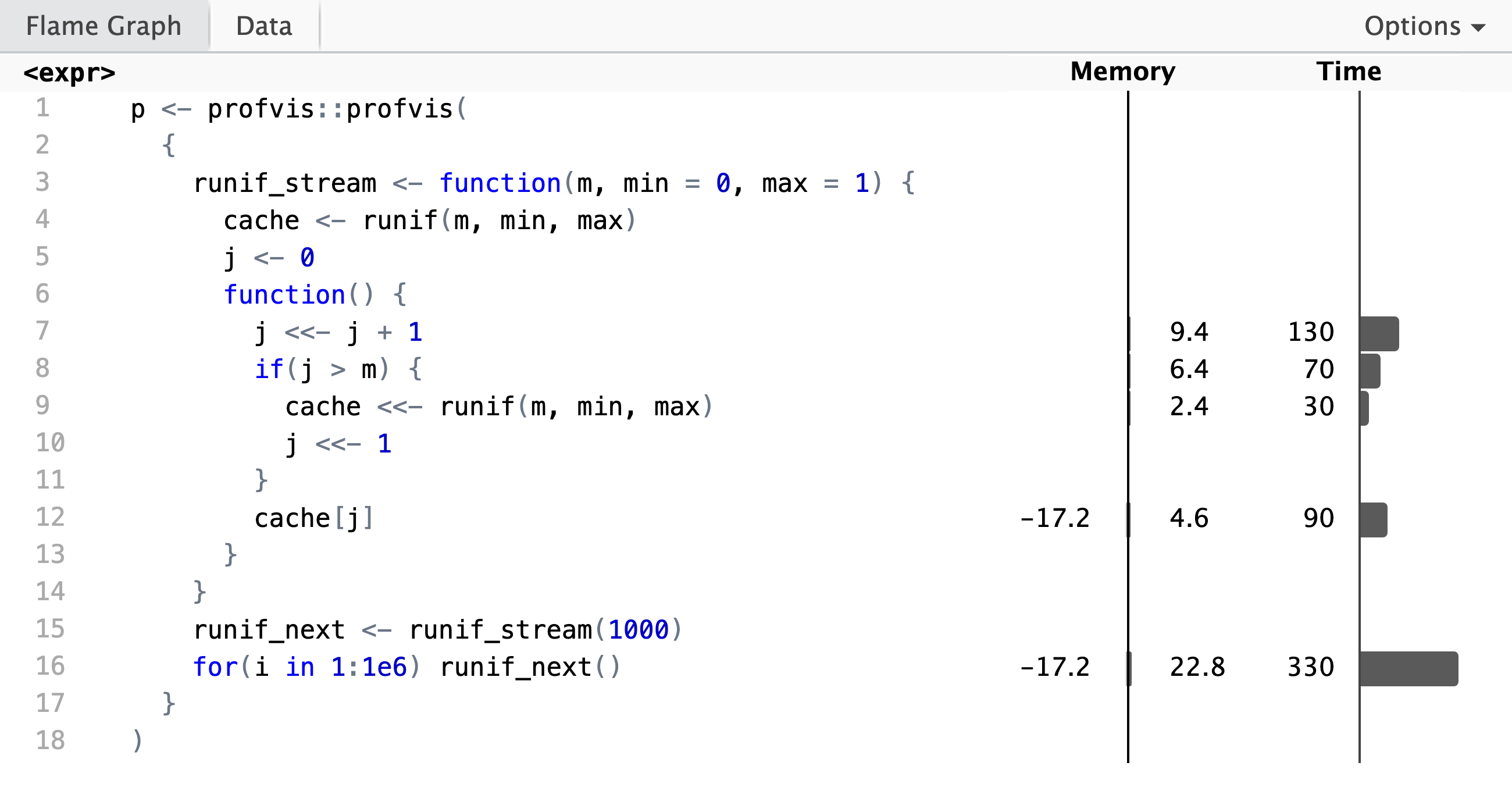
A screenshot of the HTML widget is shown below. From this we see that obtaining
five million uniformly distributed numbers generated in batches of 1000 took
about 1500 ms in total, and we see how the time is distributed among the
different lines of code. The actual generation of the random numbers takes up
only a small fraction of the total runtime—the rest of the time was spent on
incrementing the counter, j <<- j + 1, on inequality testing j > m, or on
extracting the \(j\)-th entry from the cache, cache[j].
In addition to the visual summary above, the interactive
HTML widget shows the data in the form of a
flame graph, and it includes an alternative summarized view
of the profiling data. The profiling data itself is collected by
profvis() via the Rprof() function from the utils package.
The main advantage of using profvis() is the way it processes and formats the
data—see ?Rprof to understand how the profiler actually works.
For profvis() to connect the profiling data to lines of code it must have
access to the source code. In the example above the source code of
runif_stream() was passed on to profvis() within a single R expression, but
it is also possible to profile the evaluation of a function without passing the
entire source code of that function as part of the expression. If the source
code of runif_stream() is in a file, which is read into R via the source()
function (with option keep.source = TRUE), then calling
profvis(for(i in 1:1e6) runif_next()) will give us the same profiling data as
shown above. Note that the code has to be read from the file using source()
and not copy-pasted! Note also that for the profiler to provide meaningful data,
the total evaluation time has to be long enough. That is why we do a million
evaluations of runif_next() in a loop instead of just a single one.
To illustrate the use of the profiler with sourced code, we reconsider the different implementations of the Gaussian kernel from Section A.2.
source("scripts/gauss.R", keep.source = TRUE)
x <- rnorm(10000) # Test data
# Forcing JIT, see explanation below
gauss(x)
gauss_step(x)
gauss_step_alt(x)
The script gauss.R contains the implementation of three functions. The
gauss() and gauss_step() as in Section A.2 and then
gauss_step_alt(), which is similar to gauss_step() but with a small
reorganization of some arithmetic operations. After sourcing the script, but
before running the profiler, all functions are evaluated once. This is done to
trigger the just-in-time (JIT) compilation of the functions to byte code, see
?compiler::enableJIT, and thus to avoid that this compilation step is included
in the profiling. We then run the profiler, in this case with a large number of
repeated calls of each function. This will make the execution time long enough
for the profiler to be able to sample enough data.
p <- profvis::profvis({
  for (i in 1:10000) {
    gauss(x)
  }
  for (i in 1:10000) {
    gauss_step(x)
  }
  for (i in 1:10000) {
    gauss_step_alt(x)
  }
})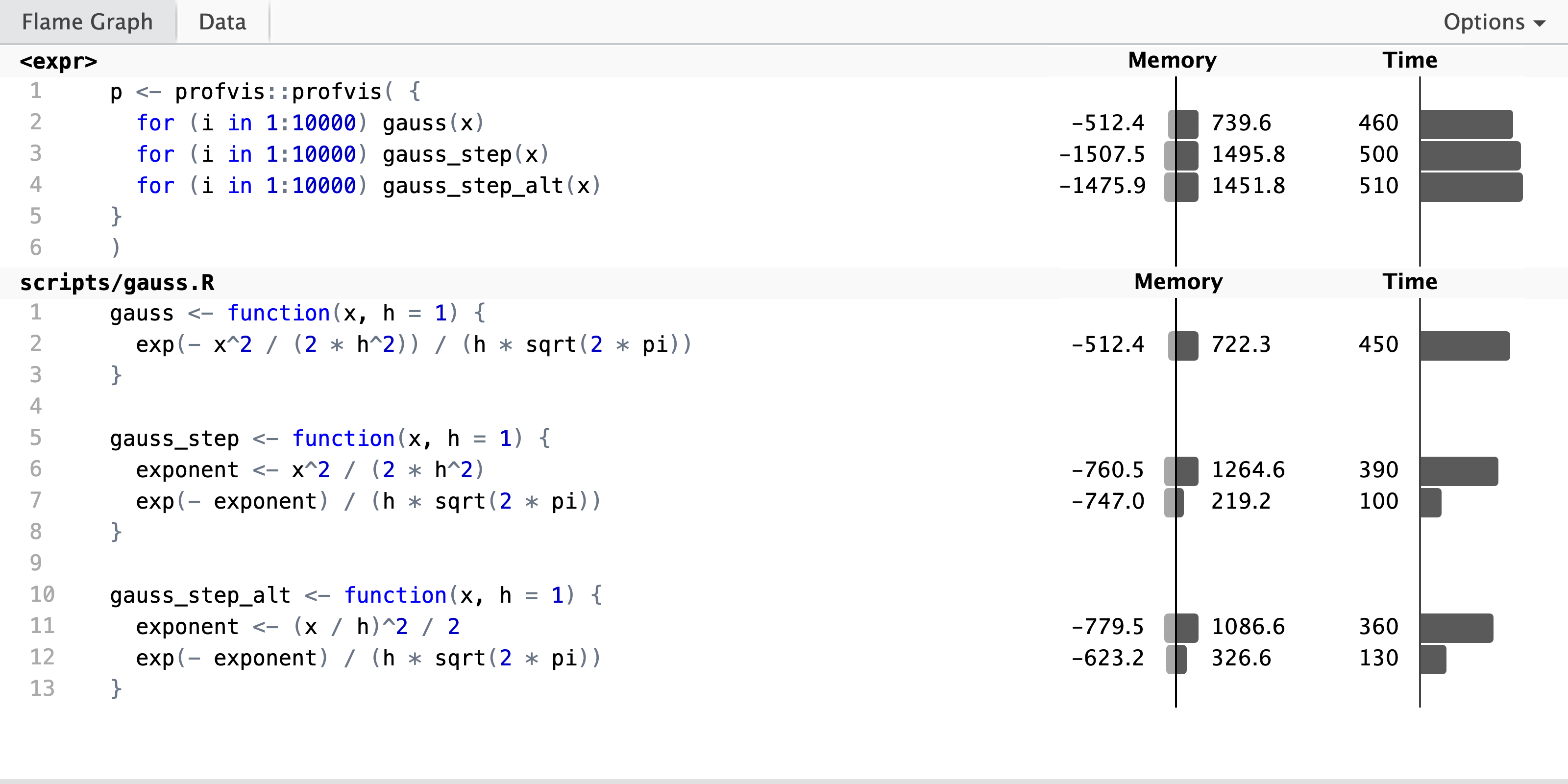
The profiling result shows that there is little difference between the three implementations in terms of runtime. The one-liner is a bit faster, probably because the step-wise solutions allocate and deallocate more memory due to the use of an extra temporary variable. From the perspective of line profiling, it is noteworthy that the two step-wise solutions give us more information about the runtime of the individual computations. Thus if you want to profile a complicated computation to understand how smaller parts of the computation affect runtime, you need to have each part of the computation on a separate line to get this information from line profiling tools.
A.3.3 Tracing
When R executes code, e.g., by evaluating a function we implemented ourselves, we would often like to peek into the interior of the function during evaluation and investigate what is going on. Besides curiosity there are two main reasons for why we want to do that. First, we might want to fix a bug. That is, when evaluating the function we get an error or a warning, or the function returns a value we know or suspect to be wrong. In those cases we need to debug the code to localize and fix the mistake(s). Second, we might want to track how a variable defined inside the body of the function evolves during the evaluation.
One pedestrian solution to the problem of peeking into a function while it is evaluated is to insert some additional code into the body of the function that can either print or store values of variables. That is, however, not a very efficient solution, and we need to remember to revert any changes we made, which can be a tedious and error-prone process.
Fortunately there are several good tools and techniques available for browsing
and tracing what is going on during a function evaluation. For one thing, R
includes debugging tools via the functions browser(), debug() and trace(),
and RStudio uses these to support debugging via visual breakpoints in the code
and it provides an interactive GUI session with access to the interior of a
function once a breakpoint is reached. We will not cover how these standard
tools are used, but they are highly recommended as much better alternatives to
debugging-by-print-statements.
What we will cover in some detail is a technique for tracing what is going on
during the evaluation of a function call, which can then be used for subsequent
analysis of the performance of an algorithm and its implementation. The
objective is to be able to store values of variables from inside a function
during normal function evaluation without altering the implementation of the
function. We present a solution based on tracer objects, created
by the tracer() function, from the CSwR package. Using these tracer objects we
can experiment with collecting any type of data during the function evaluation
without touching the implementation of the function or affecting its performance
when we are not tracing its behavior.
Using tracer objects with a function requires that we can call the object’s
tracer function inside the body of the function. It is possible to inject such a
function call into any function using the base R function trace(), and to
remove it again with the untrace() function. This can be done
programmatically, but it may be impossible to position the tracer call at the
right place this way, in which case we need to manually edit the code. This is
fine for interactive usage, but in this book we have taken a slightly different
approach. All functions we need to trace are equipped with a single so-called
callback argument, which effectively allows us to inject and
evaluate the tracer call at a particular position in the body of the function.
To illustrate the use of tracer objects we implement a function that computes the mean by a loop, which includes a callback argument.
mean_loop <- function(x, cb) {
  n <- length(x)
  x_sum <- 0
  for (i in seq_along(x)) {
    if (!missing(cb)) {
      cb()
    } # Callback
    x_sum <- x_sum + x[i]
  }
  x_sum / n
}
If any callback function is passed to mean_loop() via the cb argument it is
called in each iteration of the loop.
We proceed by constructing a tracer object with the tracer() function from the
CSwR package. Its first argument is a vector of strings specifying the names of
the variables we want to trace. Below we will trace the cumulative sum stored in
x_sum. Its second argument, Delta, specifies how often the tracer function
prints trace information during evaluation. Setting Delta = 0 means never.
Finally, when calling mean_loop() we pass the function mean_tracer$tracer()
as the callback function.
mean_tracer <- CSwR::tracer("x_sum", Delta = 100)
x <- rnorm(1000)
x_bar <- mean_loop(x, cb = mean_tracer$tracer)
## n = 1: x_sum = 0;
## n = 100: x_sum = -6.389542;
## n = 200: x_sum = 10.04348;
## n = 300: x_sum = 8.588805;
## n = 400: x_sum = 19.82415;
## n = 500: x_sum = 19.74025;
## n = 600: x_sum = 12.82393;
## n = 700: x_sum = 10.65548;
## n = 800: x_sum = 21.84324;
## n = 900: x_sum = 34.99323;
## n = 1000: x_sum = 29.21031;With Delta = 100 the tracer prints out an iteration counter and the values of
the variables being traced every 100 iterations. The complete trace is stored in
the tracer object, and it can be inspected and analyzed by converting it to a
data frame using summary().
##        x_sum        .time
## 1  0.0000000 0.000000e+00
## 2 -0.7396820 1.230044e-06
## 3  0.1718522 1.927139e-06
## 4  0.8903514 2.460321e-06
## 5  0.7941821 3.075227e-06
## 6  1.6832643 3.567198e-06
Included in the summary is the column .time, which contains the cumulative
time in seconds of each iteration. Some effort has gone into implementing the
timing of each iteration as accurately as possible. Time used by the tracer
itself is not included, and time spent on garbage collection is also excluded.
It is also possible to compute and trace additional variables not already in the
body of the function. This is done via the expr argument, which is given a
quoted expression. This expression is then evaluated in the context of the
function’s body every time the tracer is called.
mean_tracer <- tracer(
  c("x_sum", "cum_mean"),
  Delta = 100,
  expr = quote(cum_mean <- x_sum / i)
)
x <- rnorm(1000)
x_bar <- mean_loop(x, cb = mean_tracer$tracer)
## n = 1: x_sum = 0; cum_mean = 0;
## n = 100: x_sum = -11.37634; cum_mean = -0.1137634;
## n = 200: x_sum = -8.629078; cum_mean = -0.04314539;
## n = 300: x_sum = -14.95889; cum_mean = -0.04986296;
## n = 400: x_sum = -4.028055; cum_mean = -0.01007014;
## n = 500: x_sum = -11.91669; cum_mean = -0.02383338;
## n = 600: x_sum = -34.14792; cum_mean = -0.0569132;
## n = 700: x_sum = -16.84804; cum_mean = -0.02406864;
## n = 800: x_sum = -18.08451; cum_mean = -0.02260564;
## n = 900: x_sum = -30.31775; cum_mean = -0.03368639;
## n = 1000: x_sum = -45.28426; cum_mean = -0.04528426;## x_sum cum_mean .time
## 1 0.0000000 0.0000000 0.000000e+00
## 2 0.7472308 0.3736154 1.189066e-06
## 3 1.2687928 0.4229309 1.927139e-06
## 4 1.8642103 0.4660526 2.460089e-06
## 5 0.5233170 0.1046634 2.993271e-06
## 6 0.7851088 0.1308515 3.485242e-06The summary above shows that we have now also traced the cumulative mean of the
\(x\)-s. It is possible to plot the traced variables against runtime with the
autoplot() function. The default is to log-transform the time-axis, which is
not what we want in this case. The autoplot() function returns a standard
ggplot object, which can be modified as any other ggplot object. Here we add a
horizontal line at the total mean (x_bar).
autoplot(mean_tracer, cum_mean, log = FALSE) +
  geom_hline(yintercept = x_bar, color = "blue")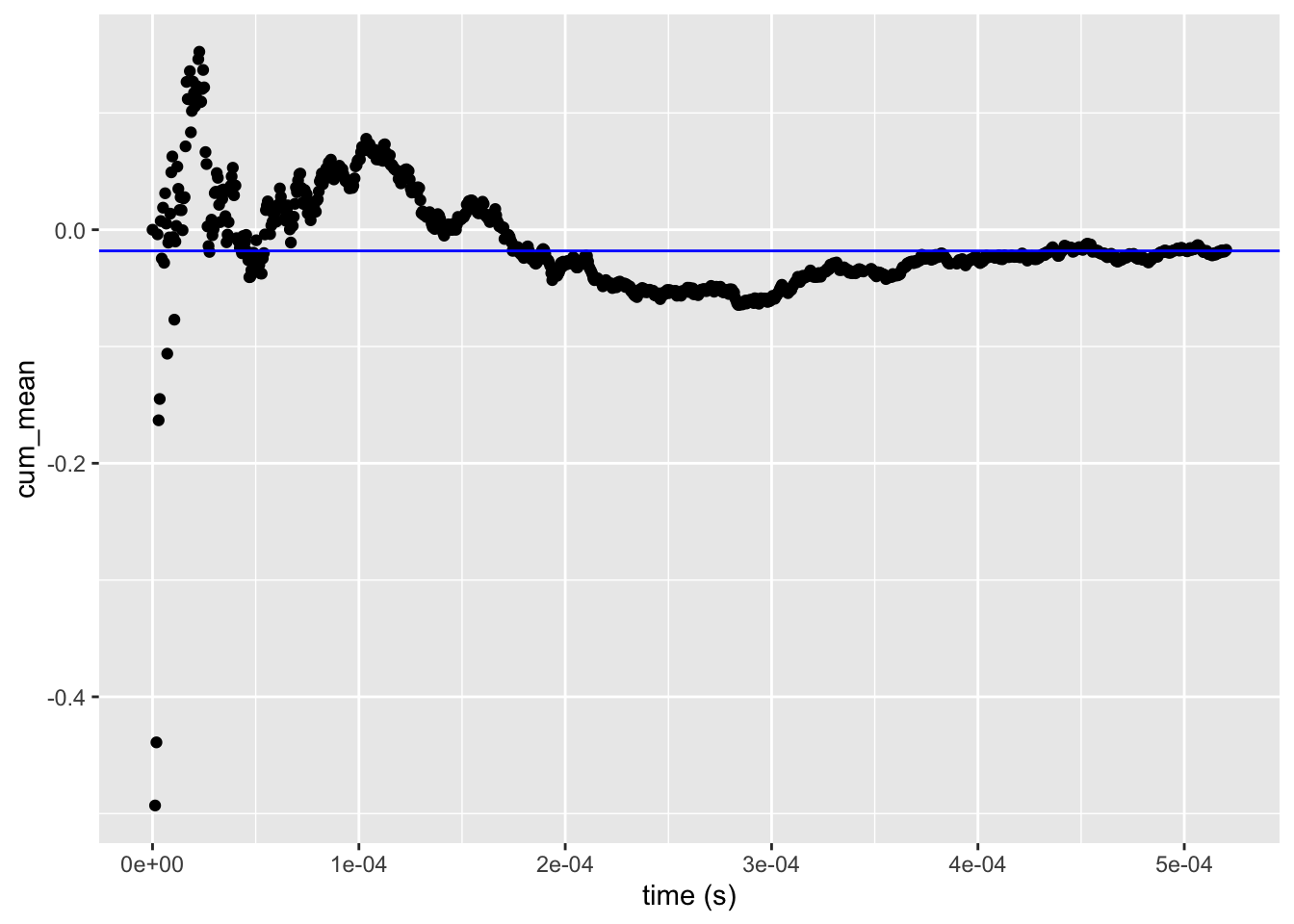
Figure A.1: Cumulative mean as a function of runtime plotted using the autoplot() method for the summary of the tracer object.
We can continue using the mean_tracer object for additional tracing, but the
information collected from earlier runs persists, and the new trace information
is just added to the object. We can, however, erase previous trace information
by calling a clear() function.
new_x <- rnorm(200)

# New trace information is added to any existing information.
x_bar <- mean_loop(new_x, cb = mean_tracer$tracer)
## n = 1100: x_sum = -19.24; cum_mean = -0.1924;
## n = 1200: x_sum = -24.6; cum_mean = -0.123;
# Clearing the trace object makes it behave as if it was just created.
mean_tracer$clear()
x_bar <- mean_loop(new_x, cb = mean_tracer$tracer)
## n = 1: x_sum = 0; cum_mean = 0;
## n = 100: x_sum = -19.24; cum_mean = -0.1924;
## n = 200: x_sum = -24.6; cum_mean = -0.123;For more information on using tracer() and tracer objects see ?CSwR::tracer.
Tracing is used throughout the book, but in particular in the chapters on
optimization. In Section A.5 we touch on the implementation of
tracer() as it relies on the S3 object system in R, and the implementation of
tracer() also uses environments extensively. The interested reader is
encouraged to study how tracer() is implemented for more insights on how
environments and function evaluation actually work in R.
A.4 Improving performance
Knuth (1974) is famous for the quote “Premature optimization is the root of all evil”—with the keyword being premature. The point is that a programmer should not in the early development process worry about all sorts of possible but minor efficiency gains. This is particularly true if such premature optimization leads to code that is more difficult to understand. Optimization is not premature once we have a working implementation and have identified our implementation’s bottlenecks. These are often minor parts of the implementation that are responsible for the majority of the runtime or memory usage. Once we have identified these parts using tools for benchmarking, profiling, and tracing our code, we can begin to optimize the implementation of the critical parts.
When we do need to optimize our R code, however, there are many techniques available for doing so. Broadly speaking, we could categorize these techniques into three categories:
- General techniques for optimizing code, which apply to any computer language, such as avoiding unnecessary copies, storing data efficiently, and parallelizing computations.
- R-specific techniques, which are based on the specific features of the R language.
- Context-specific techniques, which are based on the specific problem we are trying to solve, and include using problem-specific algorithms and data structures.
The last of these categories is often the most important one and often leads to the most significant gains. We will cover these strategies throughout the book as we go. In the sequel, we will instead focus on the former two and here provide some general guidelines for how to improve performance with respect to these.
We will start by discussing some R-specific techniques for improving performance. But first, we need to understand some basics about how R code is executed and what happens, under the hood, when you evaluate an R expression. This will help you understand why some R code is slow and how to make it faster.
When you run a piece of R code, it is not directly available in a form that the computer can execute. The reason for this is that the computer really only understands binary machine code—ones and zeros. And to make your R script executable, R needs to first interpret the code into machine code. What R does is to first parse your code into an internal representation and then dispatch your instructions to programs that already are in a binary form that the computer can execute.
This process is not unique to R in any way. Any computer language needs some kind of outer layer that translates your instructions into machine code. But how much interpretation is needed and how efficient the translation is can differ a lot between different languages. Generally speaking, the more abstract and high-level a language is, the more interpretation is needed, and R is a high-level language with complex behavior and intricate abstractions. These abstractions and features are what make R a powerful and flexible language, but it also means that R code is often quite slow.
The alternative to interpretation is compilation, which means that the translation of your code into machine code is done before you run the code. Then, at run time, the computer can “bypass” the interpretation step and directly execute the machine code. This will typically be much faster and is the reason compiled code usually outperforms interpreted code. In addition to having the binary code available, the compiler can also optimize the code during compilation, for instance by removing unnecessary computations or by rearranging computations in a more efficient way. As an added bonus, compilation also catches some types of errors early, which can be helpful for debugging.
You might wonder why we are bothering with interpreted languages (like R) at all if compiled code is both faster and safer. The reason is that interpreted languages are often much easier to write and to read than compiled languages. Compiled languages also require you to recompile your code every time you make a change, which can be a tedious process. For these reasons, it is seldom a good strategy to try to speed up your R code by rewriting all of it in a compiled language. The key strategy is instead to try to identify the bottlenecks in your R code and then to optimize those parts.
A.4.1 Using compiled functions in R
Tapping into the power of compiled code doesn’t necessarily require you to rewrite your code in a compiled language. The reason for that is that R is itself partly implemented in C, Fortran, and C++ (all compiled languages) and knowing how to tap into that power can be a very effective way to speed up your code.
For a simple example of how to tap into the power of compiled code, we can
compare the runtime of a for-loop-based implementation of the mean function with
the built-in mean().
x <- rnorm(1e6)

bench::mark(
  loop_mean = {
    x_sum <- 0

    for (i in seq_along(x)) {
      x_sum <- x_sum + x[i]
    }

    x_sum / length(x)
  },
  base_mean = mean(x)
) |>
  plot()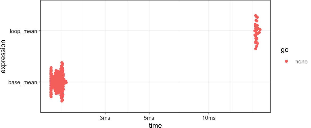
Figure A.2: Benchmarking the runtime of a simple implementation of the mean function with a for loop against the built-in mean() function, which is implemented in C.
As you can see from Figure A.2, the built-in mean() is
much faster than our simple implementation. Many people call this kind of
optimization vectorization, because it typically involves replacing loops with
vectorized functions (functions that operate on vectors, which we covered in
Vectorization)—but that statement is misleading. It is true that vectorized
functions are often much faster than R-based for loops, but the reason for that
is not that they operate on vectors or eschew the use of loops. On the contrary,
many vectorized functions are implemented with loops in C or Fortran. Moreover,
many R functions that are vectorized in fact are implemented in R-based loops,
which means that they are not faster than hand-written loops. In fact, the
opposite is often the case, as we will illustrate next.
#|
#| fig-height: 3

x <- runif(1e5, 1, 2)

bench::mark(
  loop = {
    x_log <- numeric(length(x))

    for (i in seq_along(x)) {
      x_log[i] <- log(x[i])
    }

    x_log
  },
  vapply = vapply(x, log, numeric(1))
) |>
  plot()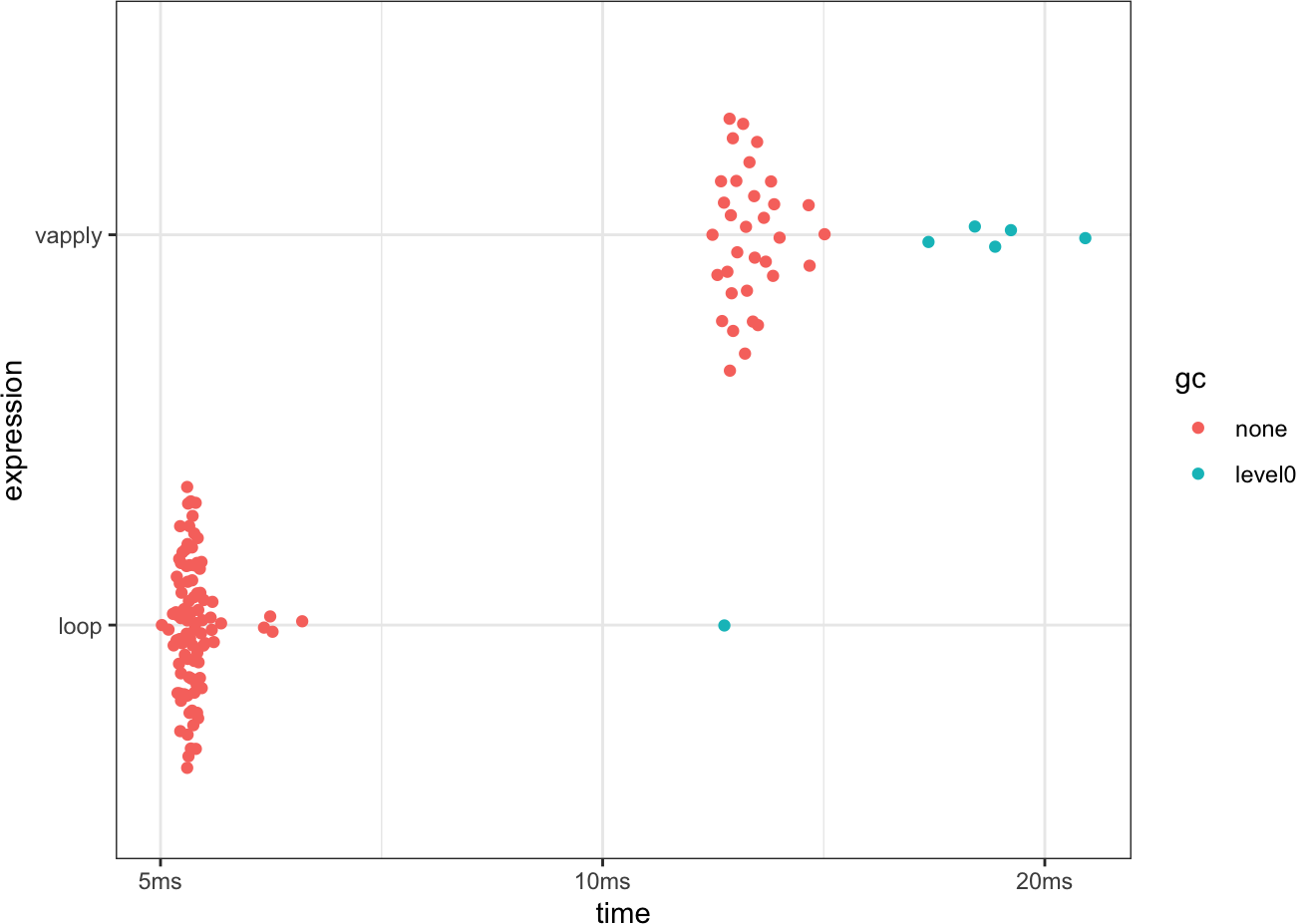
Figure A.3: Benchmarking the runtime of a for-loop-based implementation of the logarithm of a vector against an implementation using vapply(), which is a vectorized function.
Evidently, the for-loop implementation is faster than the one using vapply()
(which in turn is faster than both sapply() and lapply()). So try not to
fall into the trap of thinking that vectorization is always faster than loops.
The actual reason vectorization often helps has nothing at all to do with
vectorization itself, but is instead that vectorized functions are implemented
in a compiled language. And it is this property that we should try to profit
from.
If base R does not provide the function you need to speed up your code, you can
sometimes find it in a package instead. For instance, the
matrixStats package contains
a large number of useful functions for operating on rows and columns of
matrices, and these functions are implemented in C and are thus much faster than
R-based implementations. And if you are working on data frames, the
dplyr and
data.table packages contain a
large number of functions that are also implemented in a compiled language and
far outperform R-based implementations. So before you try to write your own
compiled code, it is often a good idea to check if there is already a package
that contains the function you need.
A.4.2 Writing compiled code in C++ with Rcpp
Sometimes the bottlenecks in our R code cannot be mitigated by relying on
existing functions in either R or external packages like matrixStats. This is
typically the case with more complicated algorithms, which often require complex
statements and control flow. Moreover, trying to wrangle R into performing well
on complicated algorithms can sometimes lead to code that is difficult to
understand and maintain. Many algorithms are, for instance, naturally expressed
with loops and if statements, and trying to avoid these can lead to obscure code
that’s both difficult to read and to debug.
In these cases, the solution is often to write the critical parts of the code in
a compiled language. R has built-in support for calling multiple compiled
languages, such as C, C++, and Fortran. Doing this with the built-in functions
.C(), .Call(), and .Fortran() is, however, far from ergonomic. Thankfully,
it is much easier to write compiled code in C++ and call it from R using the
Rcpp package (Eddelbuettel and François 2011),
which is what we will briefly introduce here.
To run the examples that follow, you need a C++ compiler installed; we cover setup in the Getting started with Rcpp section below.
We will start with an example. Consider a one-dimensional random walk that is reflected at a lower and an upper boundary: at each step, we add an increment to the current position, and if the result falls outside the interval, we mirror it back inside. Because each step depends on the previous one, this is awkward to vectorize in R, and the natural implementation uses a loop with branches.
reflected_walk_r <- function(steps, lower, upper) {
  n <- length(steps)
  x <- numeric(n + 1)

  for (i in seq_len(n)) {
    y <- x[i] + steps[i]

    if (y < lower) {
      y <- 2 * lower - y
    } else if (y > upper) {
      y <- 2 * upper - y
    }

    x[i + 1] <- y
  }

  x
}
The same algorithm in C++ using Rcpp looks like this:
#include <Rcpp.h>

// [[Rcpp::export]]
Rcpp::NumericVector
reflected_walk_cpp(Rcpp::NumericVector steps, double lower, double upper)
{
  int n = steps.size();
  Rcpp::NumericVector x(n + 1);
  x[0] = 0.0;

  for (int i = 0; i < n; ++i) {
    double y = x[i] + steps[i];

    if (y < lower) {
      y = 2 * lower - y;
    } else if (y > upper) {
      y = 2 * upper - y;
    }

    x[i + 1] = y;
  }

  return x;
}
The two implementations follow the same shape, but several syntactic differences in the C++ version stand out:
We include the Rcpp header file (
Rcpp.h) with#include <Rcpp.h>. This is similar tolibrary()in R, but we still need to explicitly include the namespace (Rcpp::) when we use functions from the Rcpp package.1We need to specify the return type of the function, which is
Rcpp::NumericVectorhere. This is a requirement of C++, which is a statically typed language, and it means that we need to declare the type of every variable we use in the function. The return type doesn’t have to go on its own line and can also be separated from the function name by a space. If your function does not return anything, you can use thevoidtype.We also need to specify argument types. Here,
stepsis anRcpp::NumericVectorandlowerandupperaredoublescalars. Local variables liken,y, and the loop counterisimilarly need their types declared.Each statement in the function body needs to end with a semicolon (
;), and the function body needs to be enclosed in curly braces ({}).The for loop is written in a C++ style, which means that we need to declare the loop variable
ias an integer and we need to specify the start, end, and step of the loop.C++ uses zero-based indexing, which means that the first element of the vector is accessed with
x[0]instead ofx[1]as in R. This is a common source of off-by-one errors when writing C++ code, so be careful with this.We need to use
returnto return the result of the function, and the returned value needs to be of the type specified in the function declaration.To assign, we use the assignment operator
=; the<-operator from R does not exist in C++.
Benchmarking the two implementations shows where Rcpp earns its keep: the compiled version is many times faster than the R loop, while remaining just as readable.
steps <- rnorm(1e5)

bench::mark(
  rcpp = reflected_walk_cpp(steps, -1, 1),
  r = reflected_walk_r(steps, -1, 1)
)
## # A tibble: 2 × 6
## expression min median `itr/sec` mem_alloc `gc/sec`
## <bch:expr> <bch:tm> <bch:tm> <dbl> <bch:byt> <dbl>
## 1 rcpp 594.34µs 694.83µs 1432. 781KB 27.9
## 2 r 7.61ms 8.01ms 125. 850KB 2.04A.4.2.1 Getting started with Rcpp
To get started with Rcpp, you need to first have a compiler installed on your system.
- Windows
-
On Windows you need to install Rtools, which is a toolchain for building R packages on Windows that includes a C++ compiler. Please see the instructions on the Rtools website for how to install it and set it up correctly.
- macOS
-
You need Xcode. Open up a terminal and call this:
- Linux
-
How to install a C++ compiler on Linux depends on the distribution you are using. On Ubuntu, you can get all the essential tools by installing the
r-base-devpackage.
To write a first Rcpp function, you can use the cppFunction() function from
the Rcpp package, which allows you to write C++ code directly in your R script.
For instance, the following code defines a simple function one() that returns
the number 1.
Rcpp::cppFunction(
  "
  int one() {
    return 1;
  }
  "
)

one()
## [1] 1This is a simple way to get started with Rcpp, but for more complicated
functions and for better organization of your code, it is better to write your
C++ code in separate files. You can then call Rcpp::sourceCpp() to source the
C++ code from a file. For instance, from a script like my_r_experiment.R, call
the following line:
Rcpp::sourceCpp("my_cpp_functions.cpp")This should work as long as the file my_cpp_functions.cpp contains valid C++
code and is in the correct location. The organization of your project could look
like this:
my_project/
├── my_r_experiment.R    # R script
├── my_cpp_functions.cpp # Source for C++ functions
└── my_rproject.Rproj    # RStudio project file
This allows you to keep your C++ code separate from your R code, which is good for organization and readability. Still, the best way to organize your code is to write an R package, which allows you to keep your code organized and to easily share it with others. We will not, however, cover how to write an R package in this book, but recommend the R Packages book (Wickham and Bryan 2023) for learning how to do that.
A.4.2.2 References
When you pass an argument in R, you typically pass a reference to the object. But if you modify the object inside the function, R will create a copy of the object and modify the copy instead. This is called copy-on-modify semantics. This is helpful because it allows you to write functions that modify their arguments without worrying about side effects while also avoiding needless copying of objects. The downside, however, is that you cannot modify an object in place, which can lead to performance issues.
C++ does not make use of copy-on-modify semantics. Instead, you need to declare
whether you want to pass an argument by value (which means that a copy of the
object is passed to the function) or by reference (which means that a reference
to the object is passed to the function). So far, we have only seen how to pass
an argument by value (copying), but if you want to pass an argument by
reference, you can do that by using the & operator in the function
declaration. For instance, the following code defines a function sum_inplace()
that takes a numeric vector as an argument and modifies it in place by adding 1
to each element.
#include <Rcpp.h>

void
sum_inplace(Rcpp::NumericVector& x)
{
  for (int i = 0; i < x.size(); ++i) {
    x[i] += 1;
  }
}
To make things slightly more complicated, there is a peculiar aspect of the Rcpp
objects that we need to be aware of: they are references to R objects, which
means that even if you omit &, they are in fact still references. This means
that you can modify them in place without using &, which can trip you up!
x <- 1.5:4.5
uh_oh(x)
x
## [1] 2.5 3.5 4.5 5.5As you can see, the uh_oh() function modifies the input vector x in place,
even though we did not use & in the function declaration. This is because
Rcpp::NumericVector is a reference to an R object, so modifying it means that
we also modify the underlying object. So be careful when modifying Rcpp objects
in place, as it can lead to unintended side effects if you are not aware of this
behavior.
In general, you should avoid modifying any Rcpp object that comes from an argument on the R side. It can absolutely be helpful for performance, but users of R are not typically used to this kind of side effect from calling a function, so it is best avoided.
A.4.3 Parallelization
Modern processors have multiple cores, which means that they can perform multiple computations simultaneously. This happens all the time when you use your computer—if it did not, just opening up a web browser or music player would freeze your computer until the program has finished loading. We can take advantage of this in our own code by splitting a computation into independent pieces and running each piece on a different core.
Parallelization is not, however, automatic. The iterations of a for loop may
depend on each other—a running sum, for instance, needs the previous value
before it can compute the next—and R cannot tell which loops are safe to
parallelize and which are not. By default, every for loop you write is
therefore executed sequentially on a single core. To run a loop in parallel we
have to mark it as such ourselves and tell R how to distribute the work.
We will use the foreach package,
which provides a near-drop-in replacement for the for loop. The idea is to
replace a loop like for (i in 1:3) { ... } with the following construct:
## [[1]]
## [1] 1
##
## [[2]]
## [1] 1.414
##
## [[3]]
## [1] 1.732
Unlike a regular for loop, foreach() returns a value—by default a list of
the results from each iteration. This is necessary because the iterations may be
executed independently and possibly out of order, so the results have to be
collected together at the end.
To run the iterations in parallel we swap %do% for %dopar%. We also need to
provide a backend: a set of worker processes that the iterations are sent to.
The parallel package, which ships with R, provides one such backend, and the
doParallel package connects
it to foreach.
library(doParallel)

cl <- makeCluster(2)
registerDoParallel(cl)

foreach(i = 1:3) %dopar% sqrt(i)
## [[1]]
## [1] 1
##
## [[2]]
## [1] 1.414
##
## [[3]]
## [1] 1.732
stopCluster(cl)Here, makeCluster(2) starts two worker R processes, registerDoParallel()
tells foreach to use them, and stopCluster() shuts them down when we are
done.
Running sqrt(i) in parallel is, of course, pointless: the cost of sending each
tiny task to a worker is much larger than the cost of computing sqrt(i).
Parallelization only pays off when each iteration does enough work to justify
this dispatch cost. As a more realistic example, consider drawing samples from a
target distribution by rejection sampling. We take the target to be the
\(\operatorname{Beta}(2, 5)\) density on \((0, 1)\) and use a uniform proposal with
envelope constant \(M = 2.5\).
beta_sample <- function(n) {
  M <- 2.5
  out <- numeric(n)
  i <- 0

  while (i < n) {
    u <- runif(1)
    if (runif(1) < dbeta(u, 2, 5) / M) {
      i <- i + 1
      out[i] <- u
    }
  }

  out
}

N <- 1e5
W <- 4
Each accept-reject decision is independent of the others, so we can split the
task of generating \(N\) samples across \(W\) workers, with each worker generating
\(N/W\) samples. Next, we compare the serial (%do%) and parallel (%dopar%)
versions.
cl <- makeCluster(W)
registerDoParallel(cl)

bench::mark(
  serial = foreach(w = 1:W, .combine = c) %do% beta_sample(N / W),
  parallel = foreach(w = 1:W, .combine = c) %dopar% beta_sample(N / W),
  check = FALSE
)
## # A tibble: 2 × 6
## expression min median `itr/sec` mem_alloc `gc/sec`
## <bch:expr> <bch:tm> <bch:tm> <dbl> <bch:byt> <dbl>
## 1 serial 378ms 380ms 2.63 1.63MB 7.89
## 2 parallel 139ms 141ms 6.90 2.13MB 0
stopCluster(cl)The parallel version is faster, but not by a factor of four. Some of the running time is spent dispatching iterations and collecting their results, and this overhead does not parallelize.
Workers started by makeCluster() are fresh R sessions and do not see the
variables or packages from your interactive session. foreach tries to
auto-detect what each iteration needs, but for non-trivial loops you may have to
pass variables and packages explicitly using the .export and .packages
arguments.
Random number generation is not synchronized between the workers and the parent
session, so setting set.seed() before a %dopar% loop does not make the
results reproducible. The doRNG
package provides a %dorng% operator that serves as a drop-in replacement for
%dopar% and produces reproducible parallel random number streams.
parallel::detectCores() reports the number of cores available on the machine,
but using all of them is rarely a good idea since the rest of the system needs
cores too. A reasonable default is to leave one or two cores free.
A.4.4 Efficient data storage and access
An often overlooked aspect of performance is how you store your data. Underneath this all lies the fact that any object that needs to persist needs to be stored somewhere in the computer’s memory. If you, for instance, need to store a vector of numbers, then you need to allocate a chunk of memory for that vector. You can think of the memory as a long row of boxes, and each box can hold a number. When you create a vector of numbers, R allocates a chunk of memory for that vector and stores the numbers in the boxes.
This memory has no sense of two-dimensionality, so even if you want to store a matrix, R needs to store its data as a long vector (plus some additional information about the dimensions of the matrix). R stores matrices in column-major order, which means that the first column of the matrix is stored in the first boxes, then the second column, and so on.
For technical reasons, accessing data that is stored in a contiguous chunk of memory is much faster than accessing data that is stored in a non-contiguous way. This means that if you want to perform operations on a matrix, it is often much faster to access the data column-wise than row-wise.
Let’s illustrate this with a simple example of matrix-vector multiplication. We will compare three different implementations of the matrix-vector product, which all compute the same result but differ in how they access the data of the matrix:
-
Take inner products between rows of the matrix and the vector.
-
Transpose the matrix and take inner products between columns of the transposed matrix and the vector.
-
Access columns of the matrix directly and update the sums together.
Now, let’s benchmark the three implementations to see how they perform.
n <- 1e3
p <- 1e1

x <- matrix(rnorm(n * p), n)
y <- matrix(rnorm(p), p, 1)

bench::mark(f1(x, y), f2(x, y), f3(x, y)) |>
  plot()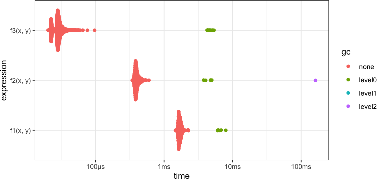
Figure A.4: Benchmark results for three different implementations of matrix-vector multiplication.
Figure A.4 shows that the first implementation, which accesses the data row-wise, is slightly slower than the second implementation, which accesses the data column-wise—even though the second implementation adds overhead from a full transpose of the matrix. But that overhead is removed from the third method, which accesses the columns directly and as a result performs best.
A.4.5 The perils and pitfalls of benchmarking
The use of benchmarking, profiling, and tracing is highly encouraged for obtaining insights about the performance of any particular implementation. The results can, however, depend on the specific configuration of the system running the code, which makes it difficult to draw general conclusions from the results.
Modern hardware and operating systems are highly complicated systems, and they continue to evolve. The same is true for the R language and any compilers used for compiling, e.g., C++ code. This means that the performance of a given implementation can vary between different hardware, operating systems, versions of R, and compilers. The issue is not that the absolute runtime of one implementation changes between different configurations, but that the relative performance of two implementations can change. This means that it can be difficult to draw general conclusions about the relative performance of an R implementation vs. a C++ implementation, say, across different configurations.
The difficulties are further compounded by a possible usage of additional and optimized libraries and the use of multiple CPU cores. The R language itself is single-threaded, but hardware-optimized libraries, such as BLAS and LAPACK for numerical linear algebra, can be multi-threaded, and they could thus use multiple CPU cores. A comparison of an R implementation that effectively relegates computations to a multi-threaded BLAS, say, with a hand-coded C++ implementation that runs on a single core is arguably a comparison of apples and oranges.
All computations, and thus all performance measurements, in the present book were done on a MacBook Pro with an M2 Max chip, running R version 4.5.2 (2025-10-31). The reference BLAS implementation shipped with R was also used. Some of the comparisons could come out differently if run with a different configuration, e.g., using Apple’s BLAS implementation from the Accelerate framework. A simple reproducibility test across platforms was done by also compiling the book on a Linux system with xx chip running Ubuntu xx, again using the reference BLAS implementation. TODO: conclusion?
With the above considerations in mind, the reader is therefore asked not to draw general conclusions from any of the specific performance comparisons. These comparisons are for the specific implementations on a specific system. They are intended to be illustrative of the process of benchmarking, profiling and tracing, and they cannot necessarily be extrapolated into general statements about the performance of R vs. C++, say.
A.5 Objects and methods
Several times in this chapter we have called the same function on different
kinds of objects and gotten behavior tailored to each. In Section A.3.3
we called summary() on a tracer object and got back a data frame of traced
values, whereas summary() of a numeric vector returns a few quantiles and
summary() of a data frame summarizes each column. Likewise, plot() rendered
a benchmark as timing distributions in Section A.3, but
plot() of two numeric vectors draws a scatterplot. Functions that adapt their
behavior to the kind of object they are given are called generic
functions, and the machinery that picks the right
behavior for the right object is R’s simplest and most widely used object
system, known as S3.
S3 is informal and lightweight. It is what the CSwR package uses for its tracer objects, and it is what we reach for whenever we want the return value of one of our own functions to print, summarize, or plot nicely instead of dumping its raw internals. The three other commonly used object systems in R, S4, R6, and S7 offer more structure and formality, but they are not used in this book and are not covered here.
We will illustrate S3 by wrapping the Gaussian kernel density estimator from Section A.2.2 in an object that carries its own evaluation grid, so that it can be printed, summarized, and plotted as a unit.
A.5.1 Classes and constructors
An S3 object is nothing more than a base object—most often a list—with a
class attribute attached. The class is a character vector, and generic
functions dispatch based on it. While we can attach a class to any object after
the fact with class<-, it is good practice to wrap the creation of an object
in a constructor function, just as it is good practice to keep any other well
defined computation in its own function (Section A.2).
The constructor below evaluates the kernel density estimator \(\overline{f}_h\) on
an equidistant grid spanning the range of the data and returns the grid, the
estimated density, the bandwidth, and the number of observations bundled
together in a list of class kde.
new_kde <- function(x, h, m = 512) {
  grid <- seq(min(x), max(x), length.out = m)
  y <- rowMeans(outer(grid, x, function(a, b) gauss(a - b, h)))

  structure(
    list(x = grid, y = y, h = h, n = length(x)),
    class = "kde"
  )
}
The structure() function is a convenient way of creating an object and setting
its attributes—here just the class—in a single call. We construct a density
estimate for the eruption durations in the faithful dataset.
dens <- new_kde(faithful$eruptions, h = 0.3)

class(dens)
## [1] "kde"
names(dens)## [1] "x" "y" "h" "n"The object dens is, underneath its class, an ordinary list, and we could
access its entries with dens$x and dens$y as for any other list. Because we
have not yet told R how a kde object should be displayed, printing dens
would simply dump all 512 grid values and densities to the console. We fix that
next.
A.5.2 Generic functions and method dispatch
print(), summary(), and plot() are all generic functions. A generic does
little on its own; its job is to inspect the class of its first argument and
hand the work over to a method—a function whose name follows the convention
generic.class. When we call print(dens), R looks for
a function called print.kde(), and if it does not find one it falls back to
print.default(). Defining a method for our class is therefore just a matter of
writing a function with the right name.
print.kde <- function(x, ...) {
  cat("Kernel density estimate\n")
  cat("  Observations:", x$n, "\n")
  cat("  Bandwidth:   ", x$h, "\n")
  cat("  Grid points: ", length(x$x), "\n")
  invisible(x)
}

dens
## Kernel density estimate
## Observations: 272
## Bandwidth: 0.3
## Grid points: 512A few conventions are worth noting. The first argument of print.kde() is
called x to match the generic print(), and the method ends with
invisible(x), which returns the object without printing it a second time—the
standard behavior for print methods. The ... argument lets the method accept
and ignore (or pass on) any further arguments, which is required because the
generic print() has a ... argument too.
The summary() generic conventionally returns a more compact representation of
an object rather than printing it. Here we return a data frame with the grid and
the estimated density, which is convenient for further computation or plotting.
summary.kde <- function(object, ...) {
  data.frame(x = object$x, density = object$y)
}

head(summary(dens))
## x density
## 1 1.600 0.2141
## 2 1.607 0.2185
## 3 1.614 0.2229
## 4 1.621 0.2273
## 5 1.627 0.2317
## 6 1.634 0.2361Note that the first argument of summary.kde() is named object, again to
match the generic summary(). Using the same argument names as the generic
ensures that arguments passed by name are matched correctly during dispatch.
A plot() method lets us visualize the object directly.
plot.kde <- function(x, ...) {
  plot(x$x, x$y, type = "l", xlab = "x", ylab = "Density", ...)
}

plot(dens)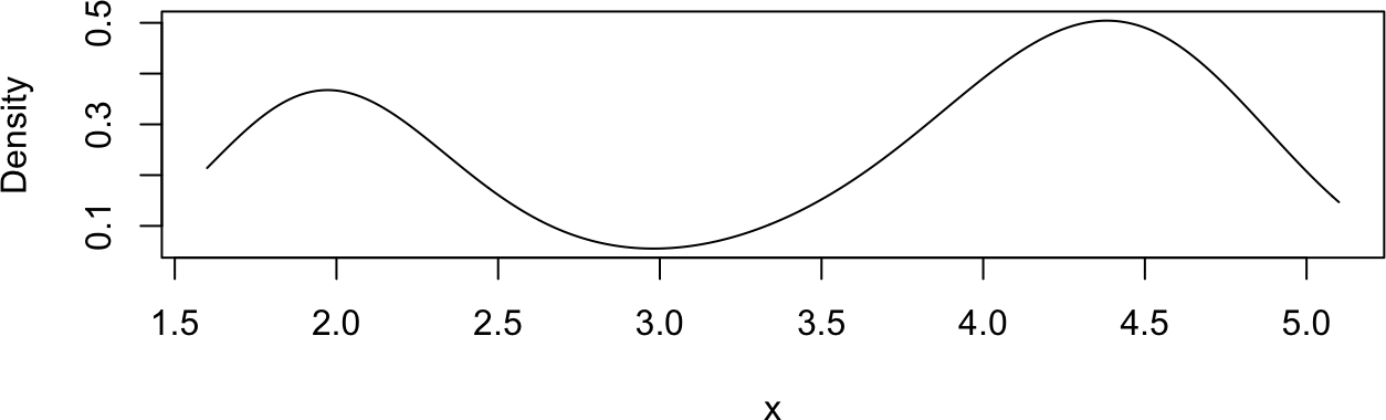
Figure A.5: The kernel density estimate plotted via the plot() method for objects of class kde.
Because the body of plot.kde() passes ... on to the inner plot() call, a
user can still set standard graphical parameters, e.g.,
plot(dens, col = "blue"), even though we never mention col in our method.
So far we have written methods for generics that already exist in R. We can just
as easily define our own generic. A generic is a function whose body consists of
a call to UseMethod() with the name of the generic. The
following peak() generic returns, for a kde object, the location of the
highest mode of the density.
peak <- function(object, ...) {
  UseMethod("peak")
}

peak.default <- function(object, ...) {
  stop("no 'peak' method for objects of class ", class(object)[1])
}

peak.kde <- function(object, ...) {
  object$x[which.max(object$y)]
}

peak(dens)
## [1] 4.381The peak.default() method is called for any object without a more specific
method, and here it simply raises an informative error. Defining a sensible
default—or a default that fails with a clear message—is good practice when
you write a generic.
A.5.3 Inheritance
The class attribute can be a vector of more than one class, and this is how S3 expresses inheritance. When dispatching, R tries each class in turn from left to right and uses the first matching method it finds. This makes it possible to give an object specialized behavior for some generics while letting it fall back on an existing class for others.
A typical situation is that we want an object to print in our own way but
otherwise behave like an object from a class that R already knows how to handle.
The hist() function, for instance, returns an object of class histogram for
which the graphics package already provides a plot() method.
## [1] "histogram"
# Prepend our own class in front of the existing one
class(h) <- c("brief_histogram", "histogram")

print.brief_histogram <- function(x, ...) {
  cat("Histogram with", length(x$counts), "cells\n")
  invisible(x)
}

h
## Histogram with 8 cellsPrinting h now dispatches to print.brief_histogram(), because
brief_histogram comes first in the class vector. Plotting h, on the other
hand, finds no plot.brief_histogram() and falls through to plot.histogram(),
so the object still draws as an ordinary histogram.
plot(h)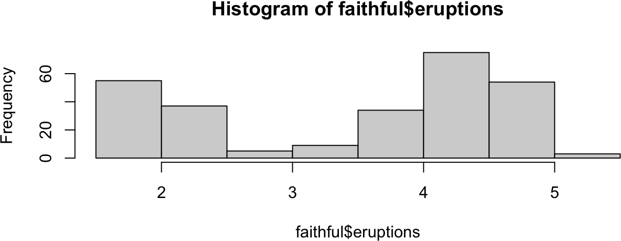
Figure A.6: An object of class c('brief_histogram', 'histogram') still plots via the inherited plot.histogram() method.
A method can also explicitly hand off to the next class in the vector by calling
NextMethod(), which is useful when our method should add
something and then defer the rest of the work to the inherited method. The
function inherits() tests whether an object has a given class, e.g.,
inherits(h, "histogram") returns TRUE.
A.5.4 S3 in the wild
The tracer objects from Section A.3.3 are a real example of everything above. A tracer is an S3 object, and the calls we made earlier dispatched to methods written for its class.
## [1] "tracer"When we wrote summary(mean_tracer) we were calling a summary.tracer() method
that turns the stored trace into a data frame, and autoplot(mean_tracer)
dispatched to an autoplot.tracer() method. The autoplot() generic is itself
defined by the ggplot2 package rather than by base R, which illustrates that we
can write methods for generics from any package, not just the base generics like
print() and summary(). Reading the implementation of tracer() in the CSwR
package is a good way to see how S3 methods, generics, and environments (Section
A.2.3) work together in a small but realistic piece of code.
A.6 Exercises
Functions
Exercise A.1 Explain the result of evaluating the following R expression.
(0.1 + 0.1 + 0.1) > 0.3## [1] TRUEExercise A.2 Write a function that takes a numeric vector x and a threshold value h as
arguments and returns the vector of all values in x greater than h. Test the
function on seq(0, 1, 0.1) with threshold 0.3. Have the example from Exercise
A.1 in mind.
Exercise A.3 Investigate how your function from Exercise A.2 treats
missing values (NA), infinite values (Inf and -Inf) and the special value
“Not a Number” (NaN). Rewrite your function (if necessary) to exclude all or
some of such values from x.
Hint: The functions is.na, is.nan and is.finite are useful.
Histograms with non-equidistant breaks
The following three exercises will use a dataset consisting of measurements of infrared emissions from objects outside of our galaxy. We will focus on the variable F12, which is the total 12 micron band flux density.
infrared <- read.table("data/infrared.txt", header = TRUE)
F12 <- infrared$F12
The purpose of this exercise is two-fold. First, you will get familiar with the data and see how different choices of visualizations using histograms can affect your interpretation of the data. Second, you will learn more about how to write functions in R and gain a better understanding of how they work.
Exercise A.4 Plot a histogram of log(F12) using the default value of the argument breaks.
Experiment with alternative values of breaks.
Exercise A.5 Write your own function, called my_breaks, which takes two arguments, x (a
vector) and h (a positive integer). Let h have default value 5. The
function should first sort x into increasing order and then return the vector
that: starts with the smallest entry in x; contains every \(h\)th unique entry
from the sorted x; ends with the largest entry in x.
For example, if h = 2 and x = c(1, 3, 2, 5, 10, 11, 1, 1, 3) the function
should return c(1, 3, 10, 11). To see this, first sort x, which gives the
vector c(1, 1, 1, 2, 3, 3, 5, 10, 11), whose unique values are
c(1, 2, 3, 5, 10, 11). Every second unique entry is c(1, 3, 10), and then
the largest entry 11 is concatenated.
Hint: The functions sort and unique can be useful.
Use your function to construct breakpoints for the histogram for different
values of h, and compare with the histograms obtained in Exercise
A.4.
Exercise A.6 If there are no ties in the dataset, the function above will produce breakpoints
with h observations in the interval between two consecutive breakpoints
(except the last two perhaps). If there are ties, the function will by
construction return unique breakpoints, but there may be more than h
observations in some intervals.
The intention is now to rewrite my_breaks so that, if possible, each interval
contains h observations.
Modify the my_breaks function with this intention and so that it has the
following properties:
- All breakpoints must be unique.
- The range of the breakpoints must cover the range of
x. - For two consecutive breakpoints, \(a\) and \(b\), there must be at least
hobservations in the interval \((a,b],\) providedh < length(x). (With the exception that for the first two breakpoints, the interval is \([a,b].\))
Functions and objects
The following exercises build on having implemented a function that computes breakpoints for a histogram either as in Exercise A.5 or as in Exercise A.6.
Exercise A.7 Write a function called my_hist, which takes a single argument h and plots a
histogram of log(F12). Extend the implementation so that any additional
argument specified when calling my_hist is passed on to hist. Investigate
and explain what happens when executing the following function calls.
my_hist()
my_hist(h = 5, freq = TRUE)
my_hist(h = 0)
Exercise A.8 Modify your my_hist function so that it returns an object of class
my_histogram, which is not plotted. Write a print method for objects of this
class, which prints just the number of cells.
Hint: It can be useful to know about the function cat.
How can you assign a class label to the returned object so that it is printed
using your new print method, but it is still plotted as a histogram when given
as argument to plot?
Exercise A.9 Write a summary method that returns a data frame with two columns containing
the midpoints of the cells and the counts.
Exercise A.10 Write a new plot method for objects of class my_histogram that uses
ggplot2 for plotting the histogram.
Functions and environments
The following exercises assume that you have implemented a my_hist function as
in Exercise A.7.
Exercise A.11 What happens if you remove that data and call my_hist subsequently? What is
the environment of my_hist? Change it to a new environment, and assign (using
the function assign) the data to a variable with an appropriate name in that
environment. Once this is done, check what now happens when calling my_hist
after the data is removed from the global environment.
Exercise A.12 Write a function that takes an argument x (the data) and returns a function,
where the returned function takes an argument h (just as my_hist) and plots
a histogram (just as my_hist). Because the return value is a function, we may
refer to the function as a function
factory.
What is the environment of the function created by the function factory? What is in the environment? Does it have any effect when calling the function whether the data is altered or removed from the global environment?
Exercise A.13 Evaluate the following function call:
tmp <- my_hist(10, plot = FALSE)What is the type and class of tmp? What happens when plot(tmp, col = "red")
is executed? How can you find help on what plot() does with an object of this
class? Specifically, how do you find the documentation for the argument col,
which is not an argument of plot()?