9 Stochastic Optimization

Numerical optimization involves different tradeoffs such as an exploration-exploitation tradeoff. On the one hand, the objective function must be thoroughly explored to build an adequate model of it. On the other hand, the model should be exploited so as to find the minimum quickly. Another tradeoff is between the accuracy of the model and the time it takes to compute with it.

The optimization algorithms considered in Chapters 7 and 8 work on all available data and take deterministic steps in each iteration. The models are based on accurate local computations of derivatives that can be greedily exploit the local model obtained from derivatives, but they do little exploration.

By including randomness into optimization algorithms it is possible to lower the computational costs and make the algorithms more exploratory. This can be done in various ways. Examples of stochastic optimization algorithms include simulated annealing and evolutionary algorithms that incorporate randomness into the iterative steps with the purpose of exploring the objective function better than a deterministic algorithm is able to. In particular, to avoid getting stuck in saddle points and to escape local minima. Stochastic gradient algorithms form another example, where descent directions are approximated by gradients from random subsets of the data.

The literature on stochastic optimization is huge, and this chapter will only cover some examples of particular relevance to statistics and machine learning. The most prominent applications are to large scale optimization, where stochastic gradient algorithms have become the standard solution. When the dimension of the optimization problem becomes very large, second order methods become prohibitively slow, and if the number of observations is also large, even one computation of the gradient for the entire data batch becomes time consuming. In those cases, stochastic gradient algorithms, that originate from online learning, can make progress more quickly while still using the entire batch of data.

9.1 Stochastic gradient algorithms

Stochastic gradient algorithms have their origin in an online learning framework, where data arrives sequentially as a stream of data points and where the objective function is an expected loss. Robbins and Monro (1951) introduced in their seminal paper a variant of the online stochastic gradient algorithm that they called the stochastic approximation method, and they established the first convergence result for such algorithms. To understand what stochastic gradient algorithms are supposed to optimize, we introduce the general framework of a population model and give conditions that ensure that the basic online algorithm converges. Subsequently, the basic online algorithm is turned into an algorithm for batch data, which is the algorithm of primary interest. In the following sections, various beneficial extensions of the basic batch algorithm are explored.

9.1.1 Population models and loss functions

We will consider observations from the sample space \(\mathcal{X}\), and we will be interested in estimating parameters from the parameter space \(\Theta\). A loss function \[L : \mathcal{X} \times \Theta \to \mathbb{R}\] is fixed throughout, and we want to minimize the expected loss also known as the risk. That is, we want to minimize \[H(\theta) = E(L(X, \theta)) = \int L(x, \theta) \mathrm{\mu}(dx)\] with \(X \in \mathcal{X}\) having distribution \(\mu\). Of course, it is implicitly understood that the expectation has to be well defined for all \(\theta\).

Example 9.1 Suppose that \(X = (Y, Z)\) with \(Y\) a real valued random variable, and that \(\mu(z, \theta)\) denotes a parametrized mean value conditionally on \(Z = z\). With the squared error loss, \[L((y,z), \theta) = \frac{1}{2} (y - \mu(z, \theta))^2,\] the risk is the mean squared error \[\mathrm{MSE}(\theta) = \frac{1}{2} E (Y - \mu(Z, \theta))^2.\] From the definition of \(\mathrm{MSE}(\theta)\) we see that \[2 \mathrm{MSE}(\theta) = E(Y - E(Y \mid Z))^2 + E (E(Y\mid Z) - \mu(Z, \theta))^2,\] where the first term does not depend upon \(\theta\). Thus minimizing the mean squared error is the same as finding \(\theta_0\) such that \(\mu(z, \theta_0)\) is the optimal approximation of \(E(Y \mid Z = z)\) in a squared error sense.

Note how the link between the distribution of \(X\) and the parameter is defined in the example above by the choice of loss function. There is no upfront assumption that \(E(Y\mid Z = z) = \mu(z, \theta_0)\) for any \(\theta_0 \in \Theta\), but if there is such a \(\theta_0\), it will clearly be a minimizer. In general, the optimal \(\theta_0\) is simply the \(\theta\) that minimizes the risk.

An alternative to the squared error loss is the log-likelihood loss, which can be used when we have a parametrized family of distributions.

Example 9.2 Suppose that \(f_{\theta}\) denotes a density on \(\mathcal{X}\) parametrized by \(\theta\). Then the log-likelihood loss is \[L(x, \theta) = - \log f_{\theta}(x).\] The corresponding risk, \[H(\theta) = - E \log(f_{\theta}(X)),\] is known as the cross-entropy. If the distribution of \(X\) has density \(f^0\) then \[\begin{align*} H(\theta) & = - E \log(f^0(X)) - E \log(f_{\theta}(X)/f^0(X)) \\ & = H(f^0) + D(f^0 \ || \ f_{\theta}) \end{align*}\] where the first term is the entropy of \(f^0\), and the second is the Kullback-Leibler divergence of \(f_{\theta}\) from \(f^0\). The entropy does not depend upon \(\theta\) and minimizing the cross-entropy is thus the same as finding a \(\theta\) with \(f_{\theta}\) being the optimal approximation of \(f^0\) in a Kullback-Leibler sense.

We consider now the same regression setup as in Example 9.1 with \(X = (Y, Z)\), but we let \[f_{\theta}(y | z) = e^{- \mu(z, \theta)} \frac{y^{\mu(z, \theta)}}{y!}\] denote the Poisson point probabilities for the Poisson distribution with mean \(\mu(z, \theta)\) conditionally on \(Z = z\). Then the log-likelihood loss is \[- \log f_{\theta}(y | z) = \mu(z, \theta) - y \log(\mu(z, \theta))\] up to an additive constant not depending on \(\theta\), and the cross-entropy is \[H(\theta) = E\big(\mu(Z, \theta) - E(Y \mid Z) \log(\mu(Z, \theta))\big),\] again up to an additive constant. This risk function quantifies how \(\mu(Z, \theta)\) deviates from \(E(Y \mid Z)\) in a different way than the risk based on the squared error loss. However, if \(E(Y \mid Z = z) = \mu(z, \theta_0)\) for some \(\theta_0\), it is still true that \(\theta_0\) is a minimizer, cf. Exercise 9.1.

The log-likelihood loss is an appropriate loss function if the parametrized family of distributions fits data well. For a Gaussian (conditional) mean value model the log-likelihood loss gives the same risk as the squared error loss – but the squared error loss can also be suitable even if data is not Gaussian. It can be a suitable loss whenever we just want to fit a model of the conditional mean of \(Y\). If we want to fit the (conditional) median instead, we can use the absolute deviation \[L((y,z), \theta) = |y - \mu(z, \theta)|.\] This is a special case of the check loss functions used for quantile regression. Thus by choosing the loss function we decide which aspects of the distribution we model, that is, whether we want a good global fit as for the log-likelihood loss, a fit of the mean value as for the squared error loss, or a fit of the the median or another quantile as for the check loss.

9.1.2 Online stochastic gradient algorithm

The classical stochastic gradient algorithm is an example of an online learning algorithm. It is based on the simple observation that if we can interchange differentiation and expectation then

\[\nabla H(\theta) = E \left( \nabla_{\theta} L(X, \theta) \right),\]

thus if \(X_1, X_2, \ldots\) form an i.i.d. sequence then \(\nabla_{\theta} L(X_i, \theta)\) is unbiased as an estimate of the gradient of \(H\) for any \(\theta\) and any \(i\). With inspiration from gradient descent algorithms it is natural to suggest stochastic parameter updates of the form

\[\theta_{n + 1} = \theta_n - \gamma_n \nabla_{\theta} L(X_{n+1}, \theta_n)\]

starting from some initial value \(\theta_0\). The direction, \(\nabla_{\theta} L(X_{n+1}, \theta_n)\), is, however, not guaranteed to be a descent direction for \(H\), and even if it is, \(\gamma_n\) is typically not chosen to guarantee descent.

The sequence of step size parameters \(\gamma_n \geq 0\) are known collectively as the learning rate. It can be a deterministic sequence, but \(\gamma_n\) may also depend on \(X_1, \ldots, X_{n}\) and \(\theta_0, \ldots, \theta_{n}\). For stochastic gradient algorithms, convergence can be shown under global conditions on the decay of the learning rate rather than local conditions on the individual step lengths.

Theorem 9.1 Suppose \(H\) is strongly convex and

\[E(\|\nabla_{\theta} L(X, \theta))\|^2) \leq A + B \|\theta\|^2.\] If

\(\theta^*\) is the global minimizer of \(H\) then \(\theta_n\) converges almost surely toward \(\theta^*\) if

\[\begin{equation} \sum_{n=1}^{\infty} \gamma_n^2 < \infty \quad \text{and} \quad \sum_{n=1}^{\infty} \gamma_n = \infty. \tag{9.1} \end{equation}\]

From the above result, convergence of the algorithm is guaranteed if the learning rate, \(\gamma_n\), converges to 0 but does so sufficiently slowly. Though formulated in a slightly different way, Robbins and Monro (1951) were the first to demonstrate convergence of an online learning algorithm under conditions as above on the learning rate. Following their terminology, much has since been written on online learning and adaptive control theory under the name stochastic approximation, Lai (2003).

The precise way that the learning rate decays is known as the decay schedule, and a flexible three-parameter power law family of decay schedules is given by

\[\gamma_n = \frac{\gamma_0 K}{K + n^a} = \frac{\gamma_0 }{1 + K^{-1} n^{a}}\]

for some initial learning rate \(\gamma_0 > 0\) and constants \(K, a > 0\). If \(a \in (0.5, 1]\) the resulting learning rate satisfies the convergence conditions (9.1).

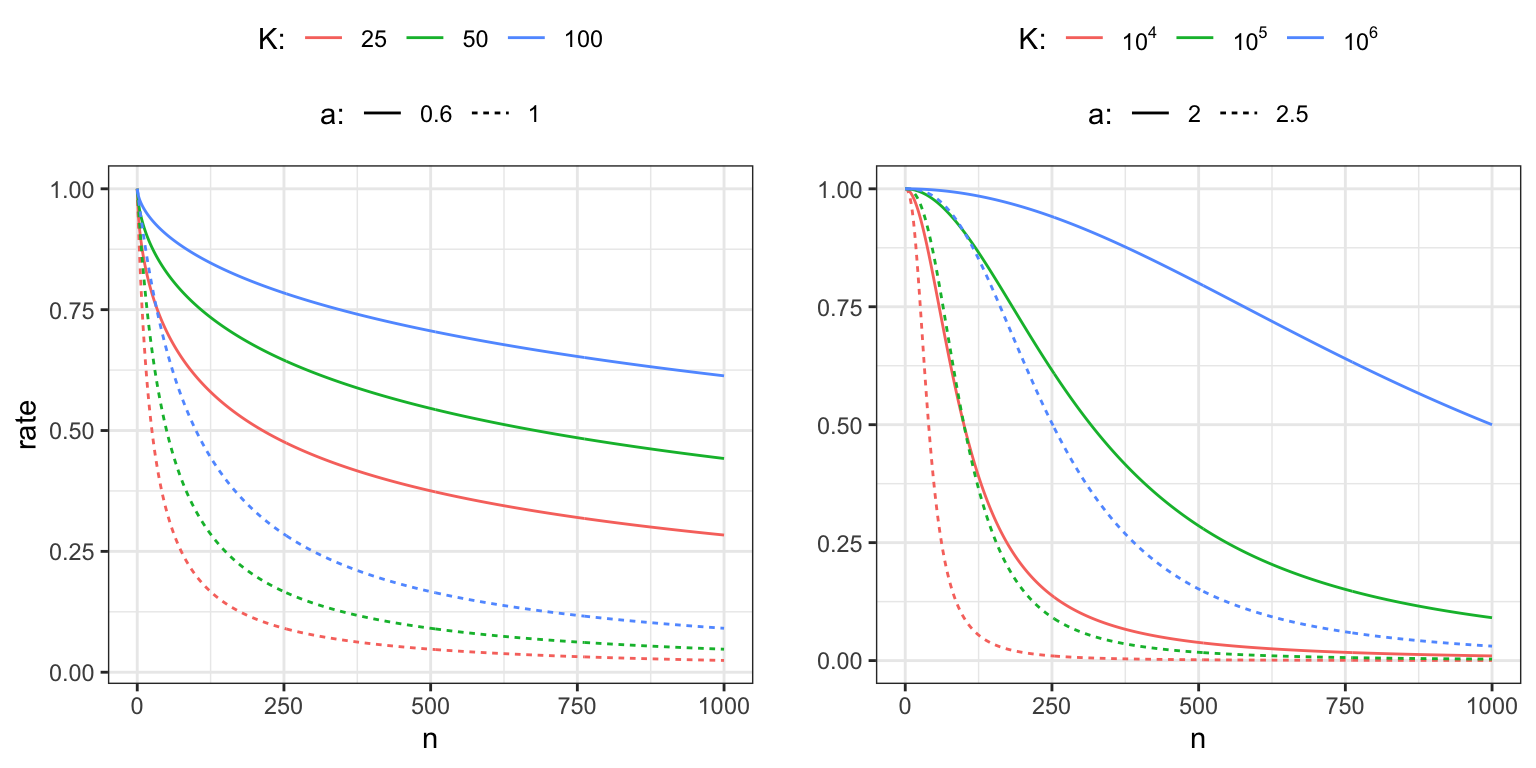
(ref:decay-fig) Power law decay schedules as a function of \(n\) for \(\gamma_0 = 1\) and for different choices of \(K\) and \(a.\) The left figure shows decay schedules with \(a\) chosen so that the convergence conditions are fulfilled, whereas the right figure shows decay schedules for which the convergence conditions are not fulfilled.

Figure 9.1: (ref:decay-fig)

The parameter \(\gamma_0\) determines the initial baseline rate, and Figure 9.1 illustrates the effect of the parameters \(K\) and \(a\) on the decay. The parameter \(a\) is the asymptotic exponent of \(\gamma_n \sim \gamma_0 K n^{-a}\), and \(K\) determines how quickly the rate will turn into a pure power law decay. Moreover, if we have a target rate, \(\gamma_{1}\), that we want to hit after \(n_{1}\) iterations, and we fix the exponent \(a\), we can also solve for \(K\) to find \[K = \frac{n_1^a \gamma_1}{\gamma_0 - \gamma_1}.\] This gives us a decay schedule that interpolates between \(\gamma_0\) and \(\gamma_1\) over the range \(0, \ldots, n_1\) of iterations.

We implement decay_scheduler() as a function that returns a particular decay schedule, with the possibility to determine \(K\) automatically from a target rate.

decay_scheduler <- function(gamma0 = 1, a = 1, K = 1, gamma1, n1) {
  force(a)
  if (!missing(gamma1) && !missing(n1))
    K <- n1^a * gamma1 / (gamma0 - gamma1)
  b <- gamma0 * K
  function(n) b / (K + n^a)
}

The following example of online Poisson regression illustrates the general ideas.

Example 9.3 In this example \(Y_i \mid Z_i = z_i \sim \mathrm{Pois}(\varphi(\beta_0 + \beta_1 z_i))\) for \(\beta = (\beta_0, \beta_1)^T\) the parameter vector and \(\varphi: \mathbb{R} \to (0,\infty)\) a continuously differentiable function. We let the \(Z_i\)-s be uniformly distributed in \((-1, 1)\), but this choice is not particularly important. The conditional mean of \(Y_i\) given \(Z_i = z_i\) is

\[\mu(z_i, \beta) = \varphi(\beta_0 + \beta_1 z_i)\] and we will first

consider the squared error loss. To this end, observe that

\[\nabla_{\beta} \mu(z_i, \beta) = \varphi'(\beta_0 + \beta_1 z_i) \left( \begin{array}{c} 1 \\ z_i \end{array} \right),\] which for the

squared error loss results in the gradient

\[\nabla_{\beta} \frac{1}{2} (y_i - \mu(z_i, \beta) )^2 = \varphi'(\beta_0 + \beta_1 z_i) (\mu(z_i, \beta) - y_i) \left( \begin{array}{c} 1 \\ z_i \end{array} \right).\]

We simulate data and explore the learning algorithm in the special case with \(\varphi = \exp\). To clearly emulate the online nature of the algorithm, the implementation below generates the observations sequentially in the loop.

N <- 5000
beta_true = c(2, 3)
mu <- function(z, beta) exp(beta[1] + beta[2] * z)
beta <- vector("list", N)

rate <- decay_scheduler(gamma0 = 0.0004, K = 100) 
beta[[1]] <- c(beta0 = 1, beta1 = 1)

for(i in 2:N) {
  # Simulating a new data point
  z <- runif(1, -1, 1)
  y <- rpois(1, mu(z, beta_true))
  # Update via squared error gradient 
  mu_old <- mu(z, beta[[i - 1]])
  beta[[i]] <- beta[[i - 1]]  - rate(i) * mu_old * (mu_old - y) * c(1, z)
}
beta[[N]]  # This is close to beta_true; the algorithm works!

## beta0 beta1 
## 2.038 2.988

For the log-likelihood loss we instead find the gradient \[\nabla_{\beta} \big( \mu(z_i, \beta) - y_i \log(\mu(z_i, \beta)) \big) = \frac{\varphi'(\beta_0 + \beta_1 z_i)}{\mu(z_i, \beta)} (\mu(z_i, \beta) - y_i) \left( \begin{array}{c} 1 \\ z_i \end{array} \right),\] which leads to a slightly different but equally valid algorithm. In the special case with \(\varphi = \exp\), the derivative is \(\varphi'(\beta_0 + \beta_1 z_i) = \mu(z_i, \beta)\), \[\nabla_{\beta} \big( \mu(z_i, \beta) - y_i \log(\mu(z_i, \beta)) \big) = (\mu(z_i, \beta) - y_i) \left( \begin{array}{c} 1 \\ z_i \end{array} \right),\] and the log-likelihood gradient differs from the squared error gradient by lacking the factor \(\mu(z_i, \beta)\). With \(Z\) uniformly distributed on \((-1, 1\)), the distribution of \(\mu(Z, (2, 3))\) has range between \(e^{-1} \simeq 0.3679\) and \(e^5 \simeq 148.4\) and is right skewed, that is, it is concentrated toward the smaller values but with a long right tail. Its median is \(e^2 \simeq 7.389\), while its mean is \((e^5 - e) / 6 \simeq 24.67\).

The squared error gradient is typically longer than the log-likelihood gradient due to the factor \(\mu(z_i, \beta)\) — and sometimes by a large factor. In the implementation below with the gradient of the log-likelihood we therefore choose \(\gamma_0\) a factor 25 larger than the \(\gamma_0 = 0.0004\) that was used with the squared error gradient.

rate <- decay_scheduler(gamma0 = 0.01, K = 100) 
beta[[1]] <- c(beta0 = 1, beta1 = 1)

for(i in 2:N) {
  # Simulating a new data point
  z <- runif(1, -1, 1)
  y <- rpois(1, mu(z, beta_true))
  # Update via log-likelihood gradient 
  mu_old <- mu(z, beta[[i - 1]])
  beta[[i]] <- beta[[i - 1]]  - rate(i) * (mu_old - y) * c(1, z)
}
beta[[N]]  # This is close to beta_true; this algorithm also works!

## beta0 beta1 
## 2.008 2.987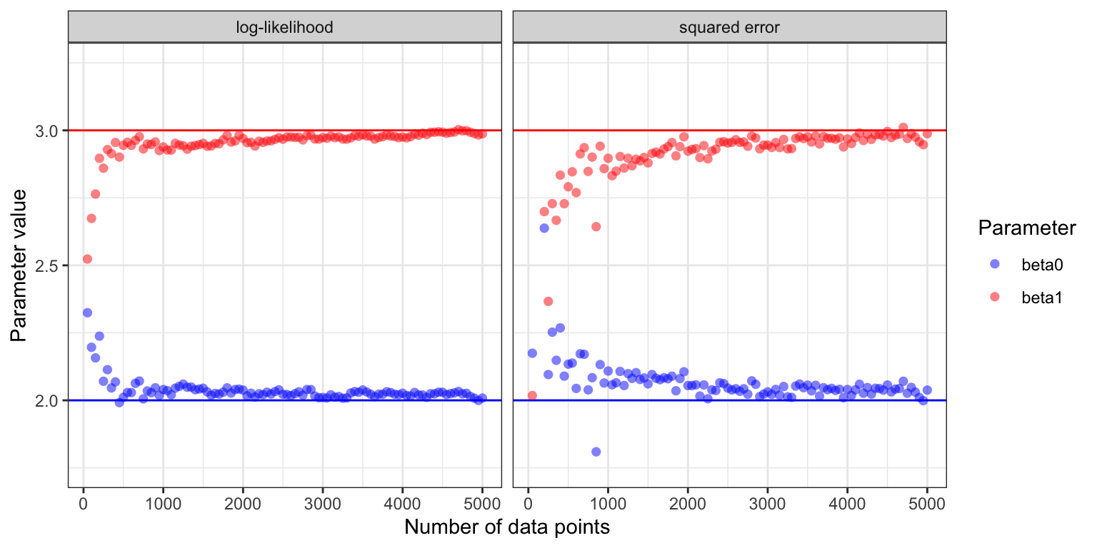

(ref:pois-sgd) Estimated parameter values for the two parameters \(\beta_0\) (true value \(2\)) and \(\beta_1\) (true value \(3\)) in the Poisson regression model as a function of the number of data points in the online stochastic gradient algorithm.

Figure 9.2: (ref:pois-sgd)

Figure 9.2 shows how the estimates of \(\beta_0\) and \(\beta_1\) converge toward the true values for the two different choices of loss functions. With \(\varphi = \exp\) and either loss function, the risk, \(H(\beta)\), is strongly convex and attains its unique minimum in \(\beta^* = (2, 3)^T\). Theorem 9.1 suggests convergence for appropriate learning rates – except that the growth condition on the gradient is not fulfilled with \(\varphi = \exp\). The growth condition is fulfilled if we replace the exponential function by softplus, \(\varphi(w) = \log(1 + e^w)\), which for small values of \(w\) behaves like the exponential function, but grows linearly with \(w\) for \(w \to \infty\).

The gradient from the squared error loss resulted in slower convergence and a more jagged sample path than the gradient from the log-likelihood. This is explained by the random factor \(\mu(z_i, \beta)\) for the squared error gradient, which makes the step sizes somewhat irregular when data is from a Poisson distribution. It also makes choosing \(\gamma_0\) a delicate balance. A small increase of \(\gamma_0\) will make the algorithm unstable, while decreasing \(\gamma_0\) will make the convergence even slower, though the fluctuations will also be damped. Making the right choice – or even a suitable choice – of decay schedule depends heavily on the problem considered and the gradient used. It is a problem specific challenge to find a good schedule – and even just to choose the three parameters when we use the power law schedule.

The example illustrates that the loss function not only determines what we model, but also how well the learning algorithm works. Both loss functions are appropriate, but since the data is from the Poisson distribution, the log-likelihood loss leads to faster convergence. Exercise 9.2 explores the opposite situation where the data is from a Gaussian distribution.

9.1.3 Batch stochastic gradient algorithms

The online algorithm does not store data, and once a data point is used it is forgotten. The online algorithm is working in a context where data arrives as a stream of data points and the model is updated continually. In statistics, we more frequently encounter batch algorithms, where an entire batch of data points is stored and processed by the algorithm, and where each data point in the batch can be accessed as many times as we like. However, when the batch is sufficiently large, many standard batch algorithms are slow, and some ideas from online algorithms can beneficially be transferred to batch processing of data.

Within the population model framework in Section 9.1.1 the objective is to minimize the population risk, \(H(\theta)\), defined as the expected loss w.r.t. the probability distribution \(\mu\). For the online algorithms we imagine an endless stream of data points from \(\mu\), which can be used to ultimately minimize \(H(\theta)\). Batch algorithms replace the population quantity by an empirical surrogate — the average loss on the batch \[H_N(\theta) = \frac{1}{N} \sum_{i=1}^N L(x_i, \theta).\] Minimizing \(H_N\) as a surrogate of minimizing \(H\) is known as empirical risk minimization.

If data is i.i.d. the standard deviation of \(H_N(\theta)\) decays as \(N^{-1/2}\) with \(N\), while the run time of its computation increases as \(N\). Thus as we invest more computation time by using more data we get diminishing returns; doubling the run time will only lower the precision of \(H_N\) as an approximation of \(H\) by a factor \(1 / \sqrt{2} \simeq 0.7\). The same is, of course, true if we look at the gradient, \(\nabla H_N(\theta)\), or higher derivatives of \(H_N\).

It is not obvious that the computational costs of using the entire data set to compute the gradient, say, is worth the effort compared to using only a fraction of the data. Thus we ask if there is a better tradeoff between run time and precision by using a fraction of data points each time we compute the gradient? The stochastic gradient algorithm is one such algorithm that “cycles through the data” and uses only a random fraction of data points for each computation. In its basic version presented first, it uses only a single data point in each iteration, and it is really the same algorithm as presented in Section 9.1.2 except that the population risk is replaced by the empirical risk defined in terms of the batch data.

With \(\hat{\mu}_N = \frac{1}{N}\sum_{i=1}^N \delta_{x_i}\) denoting the empirical distribution of the batch data set, we see that

\[H_N(\theta) = \int L(x, \theta) \mu_N(\mathrm{d}x),\]

that is, the empirical risk is simply the expected loss with respect to the empirical distribution. Thus to minimize \(H_N\) we can use the online approach by sampling observations from \(\hat{\mu}_N\). This leads to the following basic version of the stochastic gradient algorithm applied to a data batch.

From an initial parameter value, \(\theta_0\), we iteratively compute the parameters as follows: given \(\theta_{n}\)

• sample an index \(i\) uniformly from \(\{1, \ldots, N\}\)
• compute \(\rho_n = \nabla_{\theta} L(x_i, \theta_{n})\)
• update the parameter \(\theta_{n+1} = \theta_{n} - \gamma_n \rho_n.\)

Note that sampling the index \(i\) is equivalent to sampling an observation from \(\hat{\mu}_N\), which in turn is the same as nonparametric bootstrapping. Just as in the online setting, the sequence of learning rates, \(\gamma_n\), is a tuning parameter of the algorithm.

We implement the basic stochastic gradient algorithm below, allowing for a user defined decay schedule of the learning rate. However, instead of implementing one long loop, we divide the iterations into epochs with each epoch consisting of \(N\) iterations. In the implementation, the maximum number of iterations is also given in terms of epochs, and the decay schedule is applied on a per epoch basis.

We also introduce a small twist on the sampling from the empirical distribution; instead of sampling with replacement (bootstrapping) we sample without replacement. Sampling \(N\) indices from \(\{1, \ldots, N\}\) without replacement is the same as sampling a permutation of the indices.

SG <- function(
  par, 
  grad,              # Function of parameter and observation index
  N,                 # Sample size
  gamma,             # Decay schedule or a fixed learning rate
  maxit = 100,     # Max epoch iterations
  sampler = sample,  # How data is resampled. Default is a random permutation
  cb = NULL, 
  ...
) {
  gamma <- if (is.function(gamma)) gamma(1:maxit) else rep(gamma, maxit) 
  for(k in 1:maxit) {
    if(!is.null(cb)) cb()
    samp <- sampler(N)   
    for(j in 1:N) {
      i <-  samp[j]
      par <- par - gamma[k] * grad(par, i, ...)
    }
  }
  par
}

One epoch in the algorithm above is exactly one pass through the entire batch of data points, but in a random order. The default value of sampler = sample means that resampling is done without replacement. If we call SG() with sampler = function(N) sample(N, replace = TRUE) we would get sampling with replacement, in which case an epoch would be a pass through \(N\) data points sampled independently from the batch. Sampling with replacement will feed the stochastic gradient algorithm with i.i.d. samples from the empirical distribution. Sampling without replacement introduces some dependence. Curiously, sampling without replacement has turned out to be empirically superior to sampling with replacement, and recent theoretical results, Gürbüzbalaban, Ozdaglar, and Parrilo (2019), support that it leads to a faster rate of convergence.

We may ask if the sampling actually matters, and whether we could just leave out that part of the algorithm? In practice, data sets may come in a “bad order”, for instance in an unfortunate ordering according to one or more of its variables, and cycling through the data points in such an ordering can easily lead the algorithm astray. It is therefore important to always randomize the order of the data points somehow. A minimal amount of randomization in common use is to just do one initial random permutation, corresponding to moving samp <- sampler(N) outside of the outer for-loop above. This may be enough randomization for the algorithm to work in some cases, but the link to the convergence result for the online algorithm is lost.

Example 9.4 As a continuation of Example 9.3 we consider the batch version of Poisson regression. We will only use the log-likelihood gradient, and we first simulate a small data set with \(N = 50\) data points.

N <- 50
z <- runif(N, -1, 1)
y <- rpois(N, mu(z, beta_true))
grad_pois <- function(par, i) (mu(z[i], par) - y[i]) * c(1, z[i])

Using the grad_pois() function above, we run the stochastic gradient algorithm for 1000 epochs with a decay schedule that interpolates between \(\gamma_0 = 0.02\) and \(\gamma_1 = 0.001\).

pois_SG_tracer <- tracer("par", N = 0)
SG(
  c(0, 0), 
  grad_pois, 
  N = N, 
  gamma = decay_scheduler(gamma0 = 0.02, gamma1 = 0.001, n1 = 1000), 
  maxit = 1000, 
  cb = pois_SG_tracer$tracer
)

## [1] 1.905 3.163

The resulting parameter estimate should be compared to the maximum-likelihood estimate from an ordinary Poisson regression.

beta_hat <- coefficients(glm(y ~ z, family = poisson))

## beta_hat: 1.898 3.16

The batch version of stochastic gradient descent converges toward the minimizer, \((\hat{\beta}_0, \hat{\beta}_1)\), of the empirical risk. This is contrary to the online version that converges toward the minimizer of the theoretical risk, which in this case is \((\beta_0, \beta_1) = (2, 3)\). With a larger batch size, \((\hat{\beta}_0, \hat{\beta}_1)\) will come closer to \((2, 3)\). Figure 9.3 shows clearly how the algorithms converge toward a limit that depends on the batch size, and for \(N = 500\), this limit is much closer to the theoretical minimizer.

N <- 500
z <- runif(N, -1, 1)
y <- rpois(N, mu(z, beta_true))
pois_SG_tracer_2 <- tracer("par", N = 0)
SG(
  par = c(0, 0), 
  grad = grad_pois, 
  N = N, 
  gamma = decay_scheduler(gamma0 = 0.02, gamma1 = 0.001, n1 = 100), 
  cb = pois_SG_tracer_2$tracer
)

## [1] 1.995 3.022

beta_hat_2 <- coefficients(glm(y ~ z, family = poisson))

## beta_hat_2: 1.989 3.028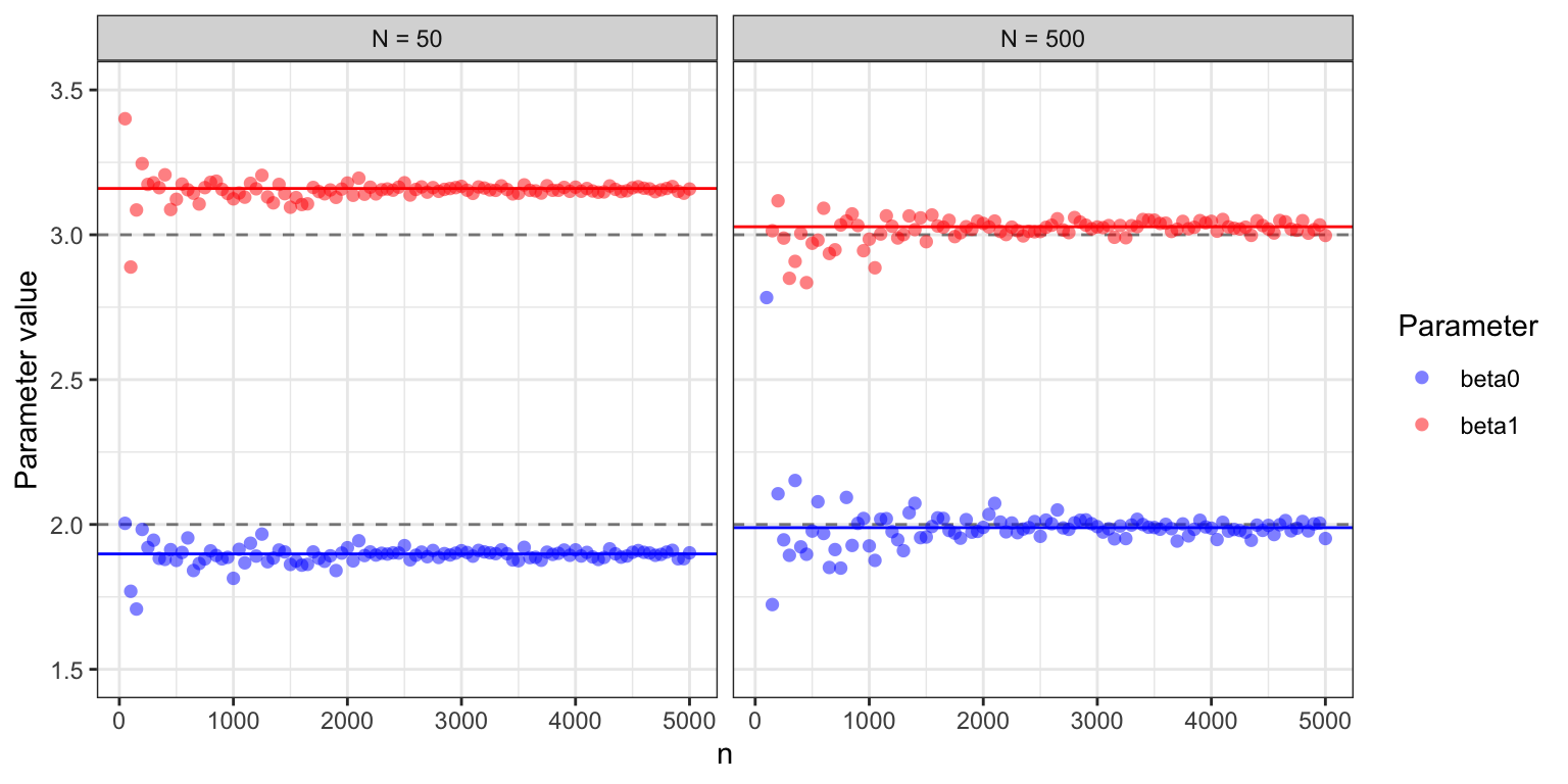

(ref:batch-pois-sgd) Estimated parameter values for the two parameters \(\beta_0 =2\) and \(\beta_1 = 3\) in the Poisson regression model as a function of the number of iterations in the stochastic gradient algorithm. For batch size \(N = 50\), the algorithm converges to a parameter clearly different from the theoretically optimal one (gray dashed lines), while for batch size \(N = 500\) the limit is closer to \((2, 3).\)

Figure 9.3: (ref:batch-pois-sgd)

Example 9.4 and Figure 9.3, in particular, illustrate that if the data set is relatively small, the algorithm quickly attains a precision smaller than the statistical uncertainty, and further optimization is therefore futile. However, for larger data sets, optimization to a greater precision can be beneficial.

9.1.4 Predicting news article sharing on social media

In this section we will illustrate the use of the basic stochastic gradient algorithm for learning a model that predicts how many times a news article is shared on social media. The data will be subjected to transformations and normalizations to make the use of a linear model and the squared error loss reasonable.

The basic stochastic gradient algorithm for the linear model was introduced to the early machine learning community in 1960 via ADALINE (Adaptive Linear Neuron) by Bernard Widrow and Ted Hoff. ADALINE was implemented as a physical device capable of learning patterns via stochastic gradient updates. The math is the same today, but the implementation has fortunately become somewhat easier.

With a linear model and the squared error loss, \(L((y, x), \beta) = \frac{1}{2} (y - \beta^T x)^2\), the gradient becomes

\[ \nabla_{\beta} L((y, x), \beta) = - x (y - \beta^T x) = x (\beta^T x - y), \]

which results in updates of the form

\[ \beta_{n+1} = \beta_n - \gamma_n x_i (\beta_n^T x_i - y_i). \]

That is, the parameter moves in the direction of \(x_i\) if \(\beta_n^T x_i < y_i\) and in the direction of \(-x_i\) if \(\beta_n^T x_i > y_i\). The amount by which it moves is controlled partly by the learning rate, \(\gamma_n\), and partly by the size of the residual, \(y_i - \beta_n^T x_i\). A larger residual gives a larger move.

The following function factory for linear models takes a model matrix and a response vector for the complete data batch as arguments and implements the squared error loss function on the entire batch as well as the gradient in a single observation. The returned list also contains a parameter vector of the correct dimension, which can be used for initialization of optimization algorithms.

ls_model <- function(X, y) {
  N <- length(y)
  X <- unname(X) # Strips X of names
  list(
    # Initial parameter value
    par0 = rep(0, ncol(X)),
    # Objective function
    H = function(beta) 
      drop(crossprod(y - X %*% beta)) / (2 * N),
    # Gradient in a single observation
    grad = function(beta, i) {  
      xi <- X[i, ]
      xi * drop(xi %*% beta - y[i])
    }
  )
}

The data, originally collected by Fernandes, Vinagre, and Cortez (2015), was obtained from the UCI Machine Learning Repository and contains 39,644 observations on 61 variables. One variable is the integer valued shares, which will be the target variable of our predictions.

News <- readr::read_csv("data/OnlineNewsPopularity.csv")

Two of the variables, timedelta and url, are not relevant predictors, and is_weekend is redundant given the other weekday variables, so we exclude those three variables. Some of the predictors are also highly correlated, and we exclude four additional predictors before the model matrix is constructed.

News <- dplyr::select(
  News,
  - url, 
  - timedelta,
  - is_weekend,
  - n_non_stop_words,
  - n_non_stop_unique_tokens,
  - self_reference_max_shares,
  - kw_min_max
)
# The model matrix without an explicit intercept is constructed from all
# variables remaining in the data set but the target variable 'shares' 
X <- model.matrix(shares ~ . - 1, data = News)  

This data set is by current standards not a large data set – the dense model matrix takes only about 20 MB of memory – and the linear model (with the target variable shares log-transformed) can easily be fitted by simply solving the least squares problem. It takes about 0.2 seconds on a standard laptop to compute the solution. The residual plot in Figure 9.4 shows that the model is actually not a poor fit to data, though there is a considerable unexplained residual variance.

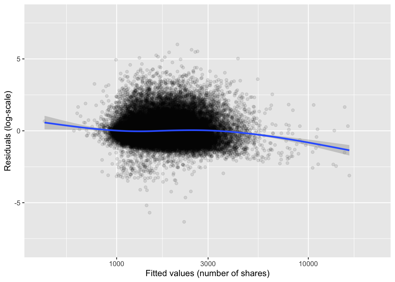
Figure 9.4: Residual plot for the linear model of the logarithm of news article shares.

Optimization of the squared error loss using this data set will be used to illustrate a number of stochastic gradient algorithms even though we can compute the optimizer easily by other means. The real practical benefit of stochastic gradient algorithms comes when applied to large scale problems that are difficult to treat as textbook examples. But using a toy problem makes it easier to understand in detail how the different algorithms behave.

We will standardize all the columns of \(X\) to have the same norm. Specifically to have non-central second moment 1. This does not change the optimization problem but corresponds to a reparametrization where all parameters are rescaled. The rescaling brings the parameters on a comparable scale, which is typically a good idea for optimization algorithms based on gradients only, see also Exercise 9.3. After rescaling we initialize the linear model with a call to ls_model() and refit the model using the new parametrization.

X_raw <- X
# Standardization and log-transforming the target variable
X <- scale(X, center = FALSE)
y <- log(News$shares)
# The '%<-%' destructure assignment operator is from the zeallot package
# c(par0, H, ls_grad) %<-% ls_model(X, y)
tmp <- ls_model(X, y)
par0 <- tmp$par0
H <- tmp$H
ls_grad <- tmp$grad
# Fitting the model using standard linear model computations
lm_News <- lm.fit(X, y)
par_hat <- lm_News$coefficients  # Will be used below for comparisons

We first run the stochastic gradient algorithm with a fixed learning rate of \(\gamma = 10^{-5}\) for 50 epochs with a tracer that computes and stores the value of the objective function at each epoch.

SG_tracer <- tracer("value", expr = quote(value <- H(par)))
SG(
  par = par0, 
  grad = ls_grad, 
  N = nrow(X), 
  gamma = 1e-5, 
  maxit = 50, 
  cb = SG_tracer$tracer
)

Using the trace from the last epochs, we can compare the objective function values to the minimum found using lm.fit() above. The minimum was not reached completely after the 50 epochs that took some time to compute.

SG_trace_low <- summary(SG_tracer)
tail(SG_trace_low)

##     value .time
## 45 0.4268 4.428
## 46 0.4263 4.528
## 47 0.4260 4.626
## 48 0.4251 4.724
## 49 0.4245 4.821
## 50 0.4240 4.919

H(par_hat)

## [1] 0.3782

We will use profiling to investigate what most of the time was spent on in the stochastic gradient algorithm.

p <- profvis::profvis(
  SG(
    par = par0, 
    grad = ls_grad, 
    N = nrow(X), 
    gamma = 1e-5,
    maxit = 50
  )
)

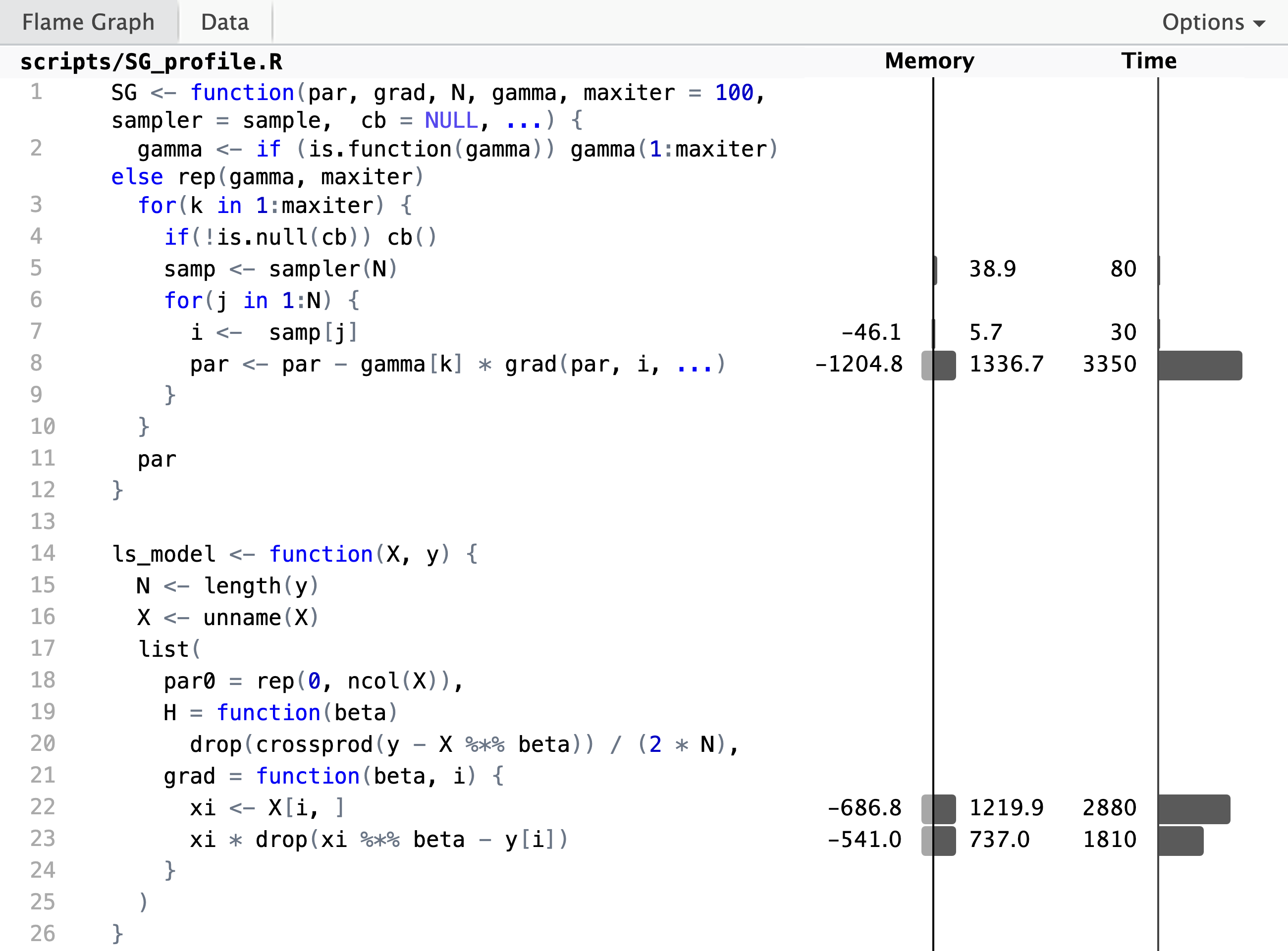
The profiling result shows, unsurprisingly, that the computation of the gradient and the update of the parameter vector takes up most of the run time. But if we look closer at the implementation of the gradient, we see that the innocuously looking subsetting X[i, ] to the \(i\)-th row is actually responsible for about half of the run time. We also see a substantial allocation and deallocation of memory associated with this line. It is a bottleneck of the R implementation that slicing out a row from a bigger matrix cannot be done without creating a copy of that row, and this is why this particular line takes up so much time.

To further investigate the convergence of the basic stochastic gradient algorithm we run it with a larger learning rate of \(\gamma = 5 \times 10^{-5}\) and then with a power law decay schedule, which interpolates from an initial learning rate of \(10^{-3}\) to a learning rate of \(10^{-5}\) after 50 epochs.

SG_tracer$clear()
SG(
  par = par0, 
  grad = ls_grad, 
  N = nrow(X), 
  gamma = 5e-5, 
  maxit= 50, 
  cb = SG_tracer$tracer
)
SG_trace_high <- summary(SG_tracer)
SG_tracer$clear()
SG(
  par = par0, 
  grad = ls_grad, 
  N = nrow(X),
  gamma = decay_scheduler(gamma0 = 7e-5, gamma1 = 4e-5, a = 0.5, n1 = 50), 
  maxit= 50, 
  cb = SG_tracer$tracer
)
SG_trace_decay <- summary(SG_tracer)

We will compare the convergence of the three stochastic gradient algorithms with the convergence of gradient descent with backtracking. For gradient descent we choose \(\gamma = 8 \times 10^{-2}\), which results in only a few initial backtracking steps and then all subsequent steps will use the step length \(\gamma = 8 \times 10^{-2}\). Choosing a larger \(\gamma\) for this particular optimization resulted in backtracking until a step length around \(8 \times 10^{-2}\) was reached, thus this choice of \(\gamma\) will use a minimal amount of time on the backtracking step of the algorithm.

grad_H <- function(beta) crossprod(X, X %*% beta - y) / nrow(X)
GD_tracer <- tracer("value", N = 10)
GD(
  par = par0, 
  H = H, 
  gr = grad_H, 
  gamma = 8e-2, 
  maxit = 800, 
  cb = GD_tracer$tracer
)
GD_trace <- summary(GD_tracer)

Figure 9.5 shows how the four algorithms converge. The gradient descent algorithm converges faster than the stochastic gradient algorithm with the low learning rate \(\gamma = 10^{-5}\), but with the high learning rate \(\gamma = 5 \times 10^{-5}\) and the power law decay schedule the stochastic gradient algorithm converges about as fast as gradient descent. For this particular run, the power law decay schedule shows marginally faster convergence than the fixed high learning rate, and this was ensured after some tuning of the decay schedule parameters. Despite
theoretical guarantees of convergence with the power law decay schedule, the practical choice of a suitable learning rate or decay schedule is really an empirical art. With very large data, the tuning of learning rate parameters can be done on a small subset of data before the algorithms are run using the full data set.

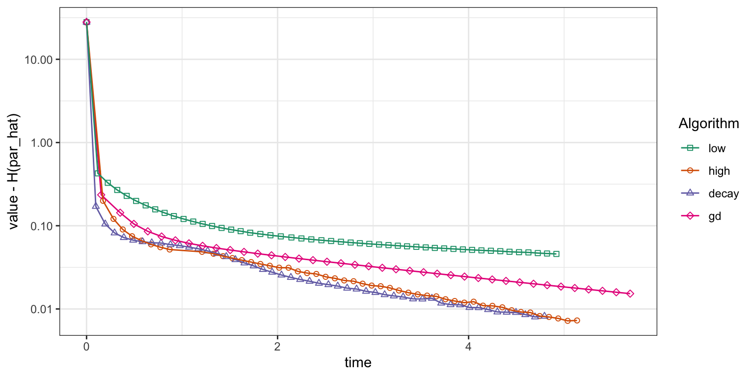
Figure 9.5: Convergence of squared error loss on the news article data set for four algorithms: gradient descent (gd) and three basic stochastic gradient algorithms with a low learning rate, a high learning rate and a power law decay schedule.

For comparison purposes it is typically better to monitor convergence of optimization algorithms as a function of real time than iterations, but when comparing algorithms in terms of real time we are admittedly comparing their specific implementations. The R implementation of the stochastic gradient algorithm has some shortcomings that are not shared by the gradient descent algorithm. One epoch of the stochastic gradient algorithm should be about as computationally demanding as one iteration of gradient descent as both will compute the gradient in each data point exactly once and add them up. The vectorized batch gradient computation is fairly efficient in R, but the iterative looping over data in the stochastic gradient algorithm is not, and this inefficiency is compounded by the inefficiency of matrix slicing that results in data copying as the profiling revealed. Thus the comparisons in Figure 9.5 are arguably not entirely fair to the stochastic gradient algorithm – only the specific R implementation.

In the subsequent section we will see alternatives to the basic stochastic gradient algorithm, which will diminish the shortcomings of a pure R implementation somewhat. Another way to circumvent some of the shortcomings of the R implementation is to rewrite the algorithm using Rcpp. We will pursue Rcpp implementations in Section 9.3, but we will first consider some beneficial modifications of the basic algorithm.

9.2 Beyond basic stochastic gradient algorithms

The gradient \(\nabla_{\theta} L(x_i, \theta)\) for a single random data point is quickly computed, and though unbiased as an estimate of \(\nabla_{\theta} H_N(\theta)\) it has a large variance. This affects the basic stochastic gradient algorithm negatively as the directions of each update can oscillate quite wildly from iteration to iteration. This section covers some techniques that yield a better tradeoff between run time and variability.

The most obvious technique is to use more than one observation per computation of the gradient, which gives us mini-batch stochastic gradient algorithms. A second technique is to incorporate some memory about previous directions into the movements of the algorithms — in the same spirit as how the conjugate gradient algorithm uses the previous gradient to modify the descent direction.

The literature on deep learning has recently exploded with variations on the stochastic gradient algorithm. Performance is mostly studied empirically and applied in practice to the highly non-convex optimization problem of learning a neural network. A comprehensive coverage of all the different ideas will not be attempted, and only three of the most solidified variations will be treated. The use of mini-batches is ubiquitous, and momentum will be introduced to illustrate a variation with memory. Finally, the Adam algorithm uses memory in combination with adaptive learning rates to achieve both speed and robustness.

9.2.1 Mini-batches

The three steps of the mini-batch stochastic gradient algorithm with mini-batch size \(m\) are: given \(\theta_{n}\)

• sample \(m\) indices, \(I_n = \{i_1, \ldots, i_m\}\), from \(\{1, \ldots, N\}\)
• compute \(\rho_n = \frac{1}{m} \sum_{i\in I_n} \nabla_{\theta} L(x_i, \theta_{n})\)
• update the parameter \(\theta_{n+1} = \theta_{n} - \gamma_n \rho_n.\)

Of course, the mini-batch algorithm with \(m = 1\) is the basic stochastic gradient algorithm. As for the basic algorithm, we implement the variation where we sample a partition \[I_1 \cup \ldots \cup I_M \subseteq \{1, \ldots, N\}\] for \(M = \lfloor N / m \rfloor\) and in one epoch loop through the mini-batches \(I_1, \ldots, I_M\).

In the following sections we will develop a couple of modifications to the basic stochastic gradient algorithm, and we will therefore implement a more generic version of the algorithm. What is common to all the modifications is that they differ in the details of the epoch loop, thus we take out that loop as a separate function.

SG <- function(
  par, 
  N,                 # Sample size
  gamma,             # Decay schedule or a fixed learning rate
  epoch = batch,     # Epoch update function
  ...,               # Other arguments passed to epoch updates
  maxit = 100,     # Max epoch iterations
  sampler = sample,  # How data is resampled. Default is a random permutation
  cb = NULL
) {
  gamma <- if (is.function(gamma)) gamma(1:maxit) else rep(gamma, maxit) 
  for(k in 1:maxit) {
    if(!is.null(cb)) cb()
    samp <- sampler(N)
    par <- epoch(par, samp, gamma[k], ...)
  }
  par
}

The implementation uses batch() as the default update function, and we implement this function below. It uses the random permutation to generate the \(M\) mini-batches, and it contains a loop through the mini-batches containing a call of grad() for the computation of the average gradient for each mini-batch in the loop. Note that the grad argument to batch() will be captured by and passed on from a call of SG() via the ... argument.

batch <- function(
    par, 
    samp,
    gamma,  
    grad,              # Function of parameter and observation index
    m = 50,            # Mini-batch size
    ...
  ) {
    M <- floor(length(samp) / m)
    for(j in 0:(M - 1)) {
      i <- samp[(j * m + 1):(j * m + m)]
      par <- par - gamma * grad(par, i, ...)
    }
    par
}

The grad() function implemented in ls_model() in Section 9.1.4 assumes that the index argument \(i\) is a single number and not a vector. It computes for a vector \(i\) a matrix containing the different gradients as columns. We therefore reimplement ls_model() so that grad() computes the average of the gradients as it is supposed to for a mini-batch.

ls_model <- function(X, y) {
  N <- length(y)
  X <- unname(X)
  list(
    par0 = rep(0, ncol(X)),
    H = function(beta)
      drop(crossprod(y - X %*% beta)) / (2 * N),
    # Gradient that works for a mini-batch indexed by i
    grad = function(beta, i) {               
      xi <- X[i, , drop = FALSE]
      drop(crossprod(xi, xi %*% beta - y[i])) / length(i)
    }
  )
}

We initialize the linear model using the new implementation of ls_model().

# c(par0, H, ls_grad) %<-% ls_model(X, y)

With increased flexibility of the algorithms comes more tuning parameters, and making a good choice of all of them becomes increasingly difficult. When introducing mini-batches we need to choose the mini-batch size in addition to the learning rate, and a good choice of learning rate or decay schedule will depend on the size of the mini-batch. To simplify matters, a mini-batch size of 1000 and a fixed learning rate are used in the subsequent applications. The learning rate will generally be chosen as large as possible without making the algorithms diverge, and with a mini-batch size of 1000 it is possible to run the algorithm with a learning rate of \(\gamma = 0.05\).

SG_tracer$clear()
SG(
  par = par0, 
  N = nrow(X), 
  gamma = 5e-2, 
  grad = ls_grad, 
  m = 1000, 
  maxit = 200, 
  cb = SG_tracer$tracer
)

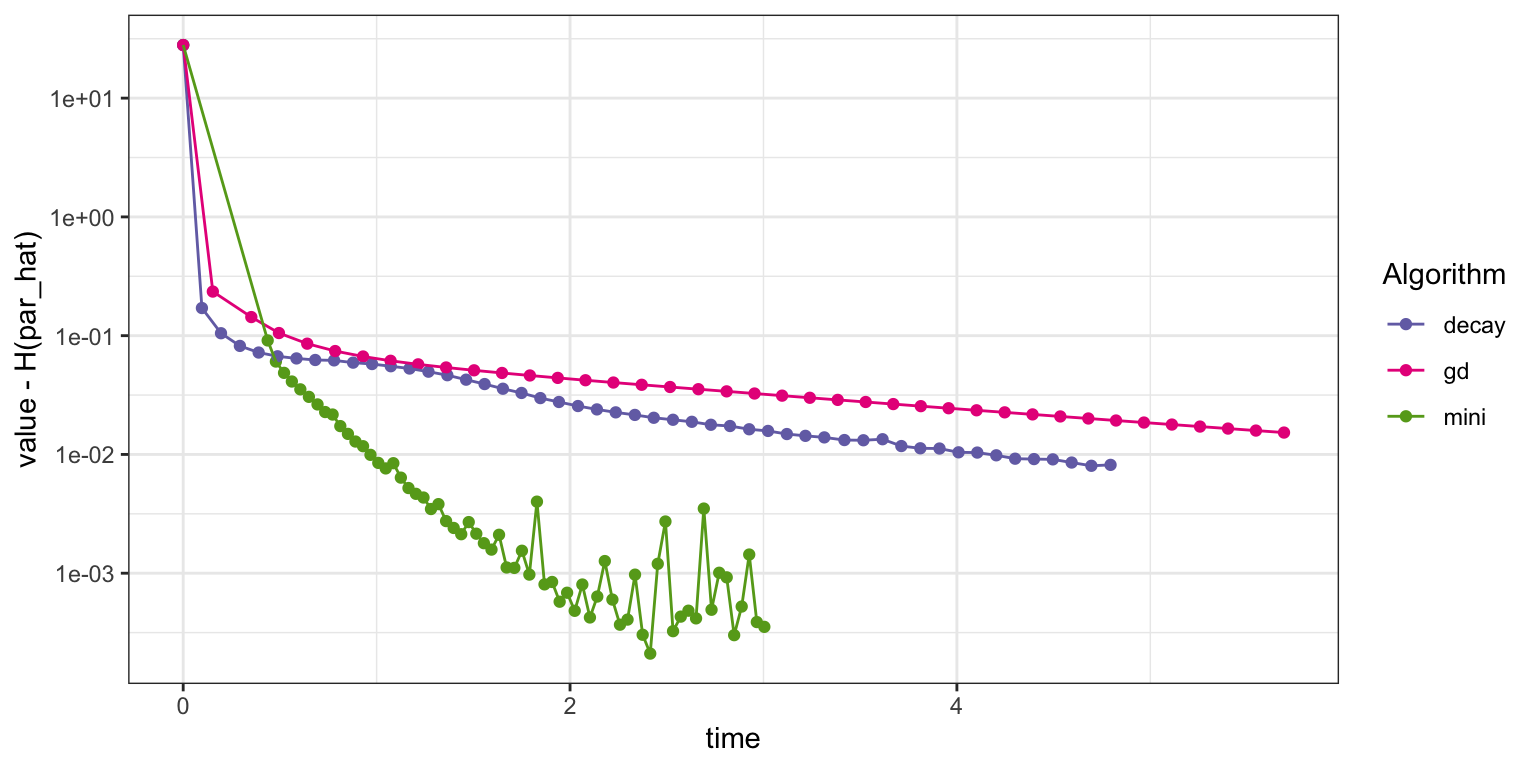
Figure 9.6: Convergence of squared error loss on the news article data set for three algorithms: basic stochastic gradient with a power law decay schedule (decay), gradient descent (gd), and mini-batch stochastic gradient with a batch size of 1000 and a fixed learning rate (mini).

Figure 9.6 shows that this implementation of the mini-batch stochastic gradient algorithm converges faster than the basic stochastic gradient algorithm with a power law decay schedule as well as the gradient descent algorithm. Eventually, it begins to fluctuate due to the fixed learning rate, but it quickly gets close to the minimum. We should not jump to conclusions from this assessment. It only really shows the improvement to the specific R implementation of using a mini-batch algorithm, and this implementation clearly benefits from the more vectorized computations with mini-batches of size 1000. We will return to this discussion in Section 9.3.1.

9.2.2 Momentum

Mini-batches stabilize the gradients, and so does momentum. Both techniques can be used in combination, and the momentum update of a mini-batch stochastic gradient algorithm is as follows: Given \(\theta_{n}\) and a batch \(I_n \subseteq \{1, \ldots, N\}\) with \(|I_n| = m\)

• compute \(g_n = \frac{1}{m} \sum_{i\in I_n} \nabla_{\theta} L(x_i, \theta_{n})\)
• compute \(\rho_n = \beta \rho_{n-1} + (1-\beta) g_n\)
• update the parameter \(\theta_{n+1} = \theta_{n} - \gamma_n \rho_n.\)

The memory of the algorithm is in the second step, where the direction, \(\rho_{n}\), is updated using a convex combination of the previous direction, \(\rho_{n-1}\), and the mini-batch gradient, \(g_n\). Usually, the initial direction is chosen as \(\rho_0 = 0\). The parameter \(\beta \in [0,1)\) is a tuning parameter determining how long the memory is. A value like \(\beta = 0.9\) or \(\beta = 0.95\) is often recommended – otherwise the memory in the algorithm will be rather short, and the effect of using momentum will be small. A choice of \(\beta = 0\) corresponds to the mini-batch algorithm without memory.

Contrary to the batch epoch function, the momentum epoch function needs to store the previous direction between updates. It is not immediately clear how to achieve this between two epochs using the generic SG() implementation, but by implementing momentum epochs using a function factory, we can easily use an enclosing environment of the epoch function for storage.

momentum <- function() {
  rho <- 0
  function(
    par, 
    samp,
    gamma,  
    grad,
    m = 50,             # Mini-batch size
    beta = 0.95,        # Momentum memory 
    ...
  ) {
    M <- floor(length(samp) / m)
    for(j in 0:(M - 1)) {
      i <- samp[(j * m + 1):(j * m + m)]
      # Using '<<-' assigns the value to rho in the enclosing environment
      rho <<- beta * rho + (1 - beta) * grad(par, i, ...)  
      par <- par - gamma * rho
    }
    par
  }
}

When calling SG() below with epoch = momentum(), the evaluation of the function factory momentum() returns the momentum epoch function with is own local environment used to store \(\rho\). With momentum, we can increase the learning rate to \(\gamma = 7 \times 10^{-2}\).

SG_tracer$clear()
SG(
  par = par0, 
  N = nrow(X), 
  gamma = 7e-2, 
  epoch = momentum(), 
  grad = ls_grad,
  m = 1000, 
  maxit = 150, 
  cb = SG_tracer$tracer
)

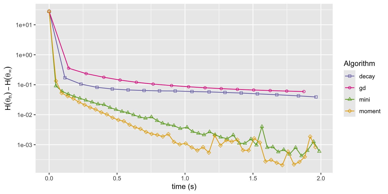
Figure 9.7: Convergence of squared error loss on the news article data set for four algorithms: gradient descent (gd), basic stochastic gradient with a power law decay schedule (decay), and mini-batch stochastic gradient with a batch size of 1000 and a fixed learning rate either without momentum (mini) or with momentum (moment).

Figure 9.7 shows that the momentum algorithm converges a little faster than the mini-batch algorithm without momentum. This can be explained by the slightly larger learning rate made possible by the use of momentum. With enough memory, momentum dampens rapid fluctuations, which allows for a larger choice of learning rate and a speedier convergence. However, too much memory results in low frequency oscillations and slow convergence. The excellent article Why Momentum Really Works contains many more details about momentum algorithms and beautiful illustrations.

9.2.3 Adaptive learning rates

One difficulty with optimization algorithms based only on gradients is that gradients are not invariant to reparametrizations. In fact, using gradients implicitly assumes that all parameters are on comparable scales. For our news article example, we standardized the model matrix to achieve this, but for many other optimization problems it is not so easy to choose a parametrization with all parameters on comparable scales. And even when we can reparametrize so that all parameters are on a common scale, this common scale can change from problem to problem making it impossible to recommend a good default choice of learning rate. The practical implication is that a considerable amount of tuning is necessary, when the algorithms are applied.

Algorithms that implement adaptive learning rates are alternatives to extensive tuning. They include schemes for adjusting the learning rate to the specific optimization problem. Adapting the learning rate is equivalent to scaling the gradient adaptively, and to achieve a form of automatic standardization of parameter scales, we will consider algorithms that adaptively scale each coordinate of the gradient separately.

To gain some intuition on how to sensibly adapt the scales of the gradient, we will analyze the typical scale of the mini-batch gradient for the linear model. Introduce first the normalized squared column norms \[\zeta_j = \frac{1}{N} \sum_{i=1}^N x_{ij}^2 = \frac{1}{N} \| x_{\cdot j}\|^2_2,\] and note that with a standardized \(X\), all the \(\zeta_j\)-s are equal. With \(\hat{\beta}\) the least squares estimate we also have that \[\frac{1}{N} \sum_{i=1}^N x_{ij} (y_i - \hat{\beta}{}^Tx_i) = 0\] for \(j = 1, \ldots, p\). Thus if we sample a random index, \(\iota\), from \(\{1, \ldots, N\}\) it holds that \(E(x_{\iota j} (y_{\iota} - \hat{\beta}{}^Tx_{\iota})) = 0\), where the expectation is w.r.t. \(\iota\). With \[\hat{\sigma}^2 = \frac{1}{N} \sum_{i=1}^N (y_i - \hat{\beta}{}^Tx_i)^2\] denoting the residual variance, we also have that

\[ V(x_{\iota j} (y_{\iota} - \hat{\beta}{}^Tx_{\iota})) = E(x_{\iota j}^2 (y_{\iota} - \hat{\beta}{}^Tx_{\iota})^2) \simeq \zeta_j \hat{\sigma}^2 \]

For the above approximation to hold, the squared residual, \((y_{\iota} - \hat{\beta}{}^Tx_{\iota})^2\), must be roughly independent of \(x_{\iota}\), which is not guaranteed by the least squares fit alone, but holds approximately if data is from a population with homogeneous residual variance.

If \(I \subseteq \{1,\ldots,N\}\) is a random subset of size \(m\) sampled with replacement, the averaged gradient \[g = - \frac{1}{m} \sum_{i \in I} x_{i} (y_i - \hat{\beta}{}^T x_i)\] is an average of \(m\) i.i.d. random variables with mean 0, thus \[E(g_j^2) = V(g_j) \simeq \zeta_j \frac{\hat{\sigma}^2}{m}.\] If \(\odot\) denotes the coordinate wise product of vectors (aka the Hadamard product), this can also be written as \[E(g \odot g) \simeq \zeta \frac{\hat{\sigma}^2}{m}.\]

The computations suggest that by estimating \(v = E(g \odot g)\) for a mini-batch gradient evaluated in \(\beta = \hat{\beta},\) we are in fact estimating \(\zeta\) up to a scale factor. We extrapolate this insight to the general case and standardize the \(j\)-th coordinate of the descent direction by an estimate of \(1 / \sqrt{v_j}\) to bring the coordinates on a (more) common scale. We will implement adaptive estimation of \(v\) using a similar update scheme as for momentum, where the estimate in iteration \(n\) is updated as a convex combination of the current value of \(g_n \odot g_n\) and the previous estimate of \(v\).

Given \(\theta_{n}\) and a batch \(I_n \subseteq \{1, \ldots, N\}\) with \(|I_n| = m\) the update consists of the following steps

• compute \(g_n = \frac{1}{m} \sum_{i\in I_n} \nabla_{\theta} L(x_i, \theta_{n})\)
• compute \(\rho_n = \beta_1 \rho_{n-1} + (1-\beta_1) g_n\)
• compute \(v_n = \beta_2 v_{n-1} + (1-\beta_2) g_n \odot g_n\)
• update the parameter \(\theta_{n+1} = \theta_{n} - \gamma_n \rho_n / (\sqrt{v_n} + 10^{-8}).\)

The vectors \(\rho_0\) and \(v_0\) are usually initialized to be \(0\). The tuning parameters \(\beta_1, \beta_2 \in [0, 1)\) control the memory of the first and second moments, respectively. The \(\sqrt{v_n}\) and the division in the last step are coordinate wise. The constant \(10^{-8}\) could, of course, be chosen differently, but is just a safeguard against division-by-zero.

The algorithm above is known as Adam (adaptive moment estimation), and was introduced and analyzed by Kingma and Ba (2014). They include so-called bias-correction steps that upscale \(\rho_n\) and \(v_n\) by the factors \(1 / (1 - \beta_1^n)\) and \(1 / (1 - \beta_2^n)\), respectively. These steps are not difficult to implement but are left out in the implementation below for simplicity. It is also possible to replace the \(\sqrt{v_n}\) by other powers \(v_n^q\). The choice of \(q = 1\) instead of \(q = 1/2\) makes the algorithm (more) invariant to scale changes. Again, for simplicity we will only implement the algorithm with \(q = 1/2\).

The adam() function below is a function factory just as momentum(), which returns a function doing the Adam epoch update loop with an enclosing environment used for storage of rho and v.

adam <- function() {
  rho <- v <- 0
  function(
    par, 
    samp,
    gamma,   
    grad,
    m = 50,          # Mini-batch size
    beta1 = 0.9,     # Momentum memory     
    beta2 = 0.9,     # Second moment memory 
    ...
  ) {
    M <- floor(length(samp) / m)
    for(j in 0:(M - 1)) {
      i <- samp[(j * m + 1):(j * m + m)]
      gr <- grad(par, i, ...) 
      rho <<- beta1 * rho + (1 - beta1) * gr 
      v <<- beta2 * v + (1 - beta2) * gr^2 
      par <- par - gamma * (rho / (sqrt(v) + 1e-8))  
    }
    par
  }
}

We run the stochastic gradient algorithm with Adam epochs and mini-batches of size 1000 with a fixed learning rate of \(0.01\) and a power law decay schedule interpolating between a learning rate of \(0.5\) and \(0.002\). The theoretical results by Kingma and Ba (2014) support a decay schedule proportional to \(1/\sqrt{n}\), thus we take \(a = 0.5\) below.

SG_tracer$clear()
SG(
  par = par0, 
  N = nrow(X), 
  gamma = 1e-2, 
  epoch = adam(), 
  grad = ls_grad,
  m = 1000, 
  maxit = 150, 
  cb = SG_tracer$tracer
)
SG_trace_adam <- summary(SG_tracer)
SG_tracer$clear()
SG(
  par = par0, 
  N = nrow(X), 
  gamma = decay_scheduler(gamma0 = 0.5, gamma1 = 2e-3, a = 0.5, n1 = 150), 
  epoch = adam(), 
  grad = ls_grad,
  m = 1000, 
  maxit = 150, 
  cb = SG_tracer$tracer
)
SG_trace_adam_decay <- summary(SG_tracer)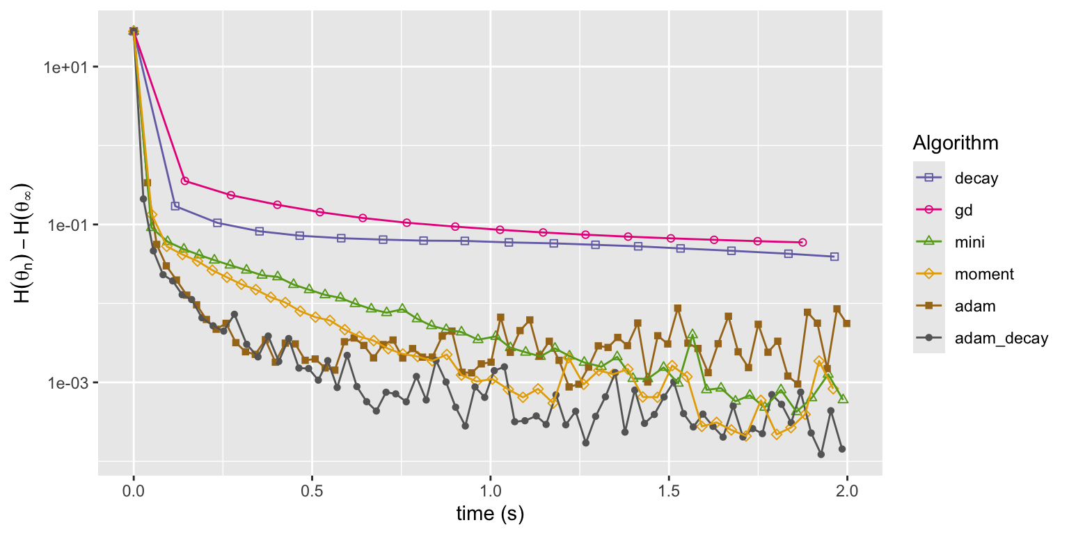

Figure 9.8: Convergence of squared error loss on the news article data set for six algorithms: basic stochastic gradient with a power law decay schedule (decay), gradient descent (gd), mini-batch stochastic gradient with a batch size of 1000 and a fixed learning rate either without momentum (mini) or with momentum (moment), and the Adam algorithm either with a fixed learning rate (adam) or a power law decay schedule (adam_decay).

Figure 9.8 shows that both runs of the Adam implementation converge faster initially than any of the other algorithms. Eventually they both level off when the error is around \(10^{-3}\) and from this point on they fluctuate randomly. What is not shown is that Adam is also somewhat more robust to changes of the learning rate and rescaling of the parameters. Though Adam has more tuning parameters, it is easier to find good values of those parameters that will lead to fast convergence.

9.3 Stochastic gradient algorithms with Rcpp

As pointed out toward the end of Section 9.1.4, the implementations of stochastic gradient algorithms in R suffer from some shortcomings. In this section we will explore how either parts of the algorithms or entire algorithms can be moved to C++ via Rcpp.

The modularity of the SG() implementation makes it easy to replace the implementation of either the gradient computation or the entire epoch loop by a C++ implementation, while retaining the overall control of the algorithm and the resampling in R. This is explored first and consists mostly of translating the numerical linear algebra of the gradient computations into C++ code. We can then easily test, compare and benchmark the implementations using the R implementation as a reference.

In the second part of this section the entire mini-batch stochastic gradient algorithm is translated into C++. This has a couple of notable consequences. First, we need access to a sampler in C++ that can do the randomization. While there are various C++ interfaces to an equivalent of sample(), some considerations need to go into an appropriate choice. Second, we have to give up on tracing as otherwise implemented. Though it is possible to implement callback of an R function from a C++ function, a tracer will not have the same access to the calling environment as in the R implementation. Thus for performance assessment we will rely on benchmarking of the entire algorithm.

For the C++ implementations we need to give up on some of the abstractions that R provides, though we will benefit from Rcpp data types like NumericVector and NumericMatrix. In a final implementation we will use RcppArmadillo to regain an abstract approach to numerical linear algebra via the C++ library Armadillo.

9.3.1 Gradients and epochs in Rcpp

We first implement the computation of the mini-batch gradient in Rcpp for the linear model, thus replacing the R implementation of the gradient in ls_model(). The implemented function takes the model matrix \(X\) and the target variable \(y\) as arguments in addition to the parameter and the subset of indices representing the mini-batch. The matrix-vector multiplications for computing predicted values, residuals and ultimately the gradient are replaced by two double for-loops.

// [[Rcpp::export]]
NumericVector lin_grad(
    NumericVector beta, 
    IntegerVector ii, 
    NumericMatrix X, 
    NumericVector y
) {
  int m = ii.length(), p = beta.length();
  NumericVector grad(p), yhat(m);
  // Shift indices one down due to zero-indexing in C++
  IntegerVector iii = clone(ii) - 1;  
  
  for(int i = 0; i < m; ++i) {
    for(int j = 0; j < p; ++j) {
      yhat[i] += X(iii[i], j) * beta[j];
    }
  }
  for(int i = 0; i < m; ++i) {
    for(int j = 0; j < p; ++j) {
      grad[j] += X(iii[i], j) * (yhat[i]- y[iii[i]]);
    }
  }
  return grad / m;
}

Note how clone(ii) is used to create a copy of the index vector ii before it is shifted by one. When R objects like vectors and matrices are passed as arguments to a C++ function, only a pointer to the data in the object is effectively passed. A modification of the resulting Rcpp object within the body of the C++ function will be reflected in R – most likely as an unwanted side effect. To prevent this we can create a copy using clone() of all data in the object – a so-called deep copy.

Since only a pointer to a matrix is passed when calling a C++ function, no notable cost is associated with passing the entire model matrix as argument. On the contrary, if we were to pass a subset of the model matrix to the C++ function from R, data would inevitably be copied. And since slicing of the matrix in C++ does not create a copy of data, the implementation of lin_grad() avoids the data copying problem that matrix slicing in R incurred on the gradient computations.

We could test lin_grad() by comparing it to ls_grad() for different choices of parameter vectors and indices. A simple way to achieve this is to run the mini-batch stochastic gradient algorithm with either implementation of the gradient for one epoch and compare the results. Note that we make sure the algorithms use the same mini-batches by setting the seed.

set.seed(10)
par1 <- SG(
  par = par0,
  grad = ls_grad,
  N = nrow(X),
  gamma = 0.01,
  maxit = 1
)
set.seed(10)
par2 <- SG(
  par = par0, 
  grad = lin_grad,
  N = nrow(X),
  gamma = 0.01,
  maxit = 1, 
  X = X,
  y = y
)
range(par1 - par2)

The differences are all 0, thus the test indicates that lin_grad() implements the same computation as ls_grad().

We can also move the entire epoch loop to C++, thus replacing the batch() R function by Rcpp function lin_batch() below. This is achieved simply by adding one outer loop to lin_grad() above, which loops over mini-batches and updates the parameter vector.

// [[Rcpp::export]]
NumericVector lin_batch(
    NumericVector par, 
    IntegerVector ii, 
    double gamma, 
    NumericMatrix X, 
    NumericVector y, 
    int m = 50
) {
  int p = par.length(), N = ii.length();
  int M = floor(N / m);
  NumericVector grad(p), yhat(N), beta = clone(par);
  IntegerVector iii = clone(ii) - 1;  
  
  for(int j = 0; j < M; ++j) {
    for(int i = j * m; i < (j + 1) * m; ++i) {
      for(int k = 0; k < p; ++k) {
        yhat[i] += X(iii[i], k) * beta[k];
      }
    }
    for(int k = 0; k < p; ++k) {
      grad[k] = 0;
      for(int i = j * m; i < (j + 1) * m; ++i) {
        grad[k] += X(iii[i], k) * (yhat[i] - y[iii[i]]);
      }
    }
    beta = beta - gamma * (grad / m);
  }
  return beta;
}

We can test the implementation of lin_batch() just as lin_grad() by running the stochastic gradient algorithm for one epoch. We note that the lin_batch() function should be passed to SG() as the epoch argument, and that no grad argument is required. The gradient computations are hard coded into the implementation of this epoch function.

set.seed(10)
par1 <- SG(
  par = par0,
  grad = ls_grad,
  N = nrow(X),
  gamma = 0.01,
  maxit = 1
)
set.seed(10)
par2 <- SG(
  par = par0, 
  epoch = lin_batch,   
  N = nrow(X),
  gamma = 0.01,
  maxit = 1, 
  X = X,
  y = y
)
range(par1 - par2)

We see that these differences are also zero, and the test indicates that lin_batch() implements the same computation as batch() with either of the two implementations of the gradient.

To investigate the effect of the C++ implementation, the mini-batch stochastic gradient algorithm is run with the Rcpp implementations of either the gradient or the entire epoch using a mini-batch size of 1000 and a constant learning rate \(\gamma = 0.05\), which can be compared to the pure R implementation. In addition, we run the algorithm with mini-batch size one and \(\gamma = 5 \times 10^{-5}\) using the Rcpp implementation of the epoch.

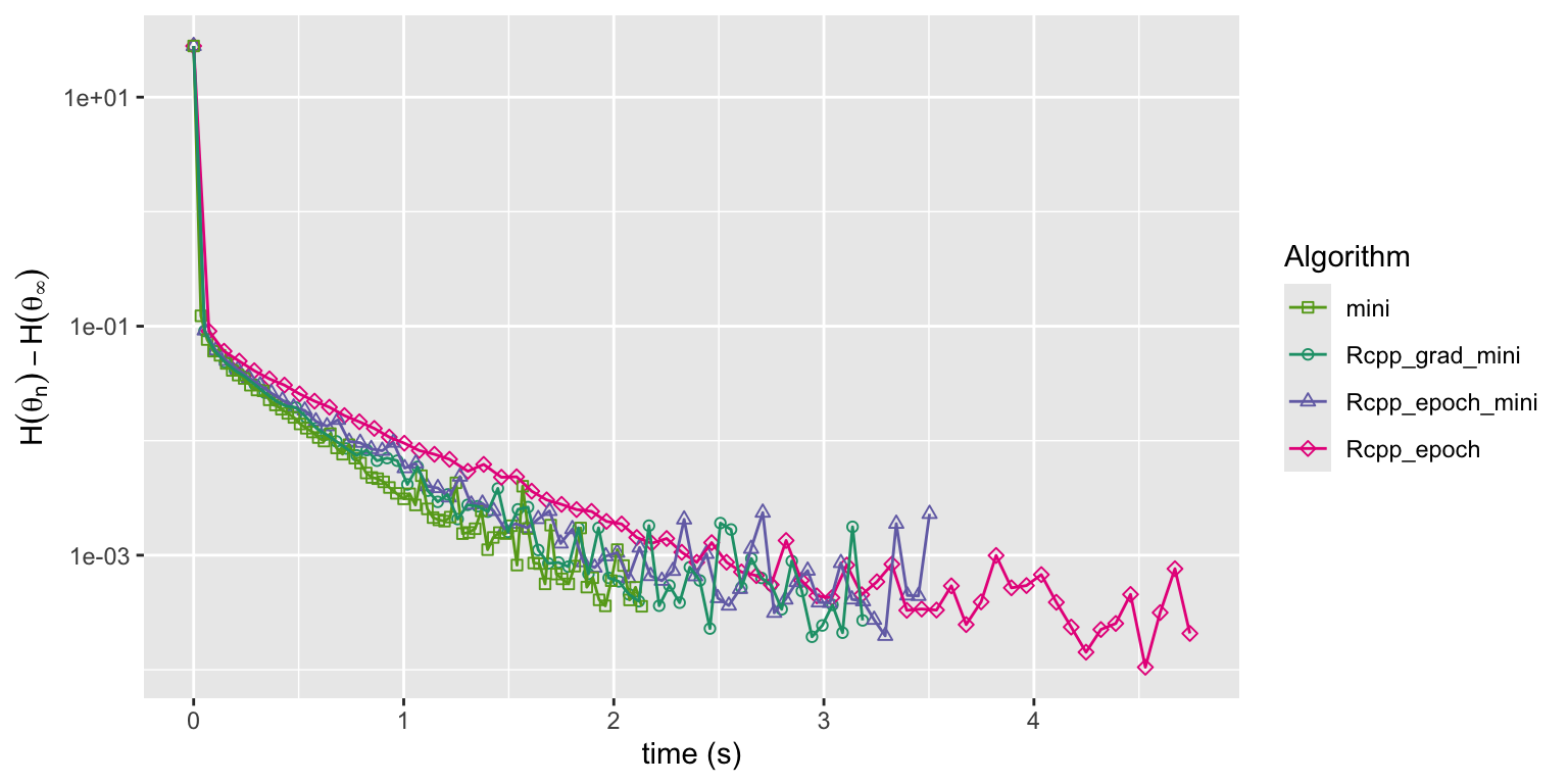
Figure 9.9: Convergence of squared error loss on the news article data set for four algorithms: R implementation of mini-batch stochastic gradient with a batch size of 1000 and a fixed learning rate (mini), the same mini-batch algorithm but with the gradient implemented in Rcpp (Rcpp_grad_mini) and with the entire epoch implemented in Rcpp (Rcpp_epoch_mini), and the basic stochastic gradient algorithm with the entire epoch implemented in Rcpp (Rcpp_epoch).

Figure 9.9 shows, unsurprisingly, that implementing the gradient as a C++ function makes the convergence faster compared to the pure R implementation, but turning the entire epoch into a C++ function results in little if any further improvement. However, the figure also shows that the basic stochastic gradient algorithm (mini-batch size equal to one) converges at a rate comparable to that of the mini-batch algorithm with mini-batch size 1000 when the entire epoch is in C++. Thus any benefit of the mini-batch algorithm with mini-batch size 1000 seems to be largely due to the inefficiency of the basic algorithm in pure R. Experiments using the lin_batch() epoch implementation (not shown) suggest that the mini-batch algorithm does have a real edge over the basic algorithm, but with much smaller mini-batch sizes, e.g. \(m = 20\), cf Exercise 9.4.

9.3.2 Full Rcpp implementations

In this section we convert the entire stochastic gradient algorithm for the linear model into a C++ function. Two considerations come up when doing so:

• How do we sample with or without replacement in C++?
• Is it possible in C++ to implement the gradient computations using numerical linear algebra instead of two double for-loops?

We deal with the first question first, that is, how to sample from a finite set of size \(d\) in C++ such as sample() does in R. Though it may seem like a rather trivial problem, it is not entirely trivial to implement sampling from a general distribution on a finite set of size \(d\) that is both correct and efficient as a function of \(d\). A non-exhaustive list of ways to sample from discrete sets using Rcpp is:

• The R function sample() can be retrieved via Function sample("sample"); in Rcpp, which makes the function callable from C++ code. There is, however, an overhead associated with calling R functions from C++, which we prefer to avoid.
• There is an Rcpp sugar implementation of sample(). It generates different samples than the R function sample().
• There is an RcppArmadilloExtension implementation of sample(). See also the blog post Sampling Integers. It requires the R package RcppArmadillo, and it also generates different samples than the R function sample().
• There is the function dqsample.int() from the dqrng package dealt with in Section 4.1.2. It requires the R package dqrng and runs on an independent stream of pseudo random numbers then R’s RNG.

The Rcpp sugar and the Rcpp Armadillo versions of sample() are touched on in the Rcpp introduction vignette, but they are not documented in detail. Both use R’s stream of pseudo random numbers, but they nevertheless generate sequences that differ from each other and from sample(). To reproduce results in R, we would have to write an interface to those C++ functions if we were to use them. Since the dqrng package provides an interface to dqsample.int() from R as well as from C++, we will use that sampler in our implementations.

If we only want to generate random permutations, there are a couple of additional alternatives. There is randperm() from the Armadillo library, and there is also std::random_shuffle() from the C++ Standard Library. The implementation of std::random_shuffle() is, however, not specified by the standard and can be compiler dependent. Both of these alternatives will also run on an independent stream of pseudo random numbers then
R’s RNG, and will not be considered any further.

The full Rcpp implementation of the stochastic gradient algorithm is now a simple extension of lin_batch() with one additional outer loop over the epochs and a single line calling dqsample_int() to sample the random permutation.

// [[Rcpp::depends(dqrng)]]
// [[Rcpp::export]]
NumericVector SG_Rcpp(
    NumericVector par, 
    int N, 
    NumericVector gamma,
    NumericMatrix X, 
    NumericVector y,
    int m = 50, 
    int maxit = 100
) {
  int p = par.length(), M = floor(N / m);
  NumericVector grad(p), yhat(N), beta = clone(par);
  IntegerVector ii;
  
  for(int l = 0; l < maxit; ++l) {
    // Note that dqsample_int samples from {0, 1, ..., N - 1}
    ii = dqrng::dqsample_int(N, N); 
    for(int j = 0; j < M; ++j) {
      for(int i = j * m; i < (j + 1) * m; ++i) {
        yhat[i] = 0;
        for(int k = 0; k < p; ++k) {
          yhat[i] += X(ii[i], k) * beta[k];
        }
      }
      for(int k = 0; k < p; ++k) {
        grad[k] = 0;
        for(int i = j * m; i < (j + 1) * m; ++i) {
          grad[k] += X(ii[i], k) * (yhat[i] - y[ii[i]]);
        }
      }
      beta = beta - gamma[l] * (grad / m);
    }
  }
  return beta;
}

We test the implementation by comparing it to the pure R implementation, but using dqsample_int() / dqsample.int() to sample the same permutations in both cases.

dqset.seed(10) 
par1 <- SG(
  par = par0, 
  grad = ls_grad,
  N = nrow(X), 
  gamma = 1e-3, 
  maxit = 10,
  sampler = dqrng::dqsample.int
)
dqset.seed(10) 
par2 <- SG_Rcpp(
  par = par0, 
  N = nrow(X),
  gamma = rep(1e-3, 10),
  X = X, 
  y = y,
  maxit = 10
)
range(par1 - par2)

The two most notable overall differences between SG() and SG_Rcpp() is that SG_Rcpp() is low level and very problem specific, while SG() is high level and generic. It is surely possible to refactor the C++ code to write a more generic stochastic gradient algorithm, that would rely on other functions for computing e.g. the gradient. However, to retain performance those functions would need to be implemented in C++ as well.

To achieve a more high level implementation, we can use the RcppArmadillo package, which provides an interface to numerical linear algebra from the C++ library Armadillo. In this way we can use a matrix-vector style implementation similar to the R implementation but without excessive data copying. It is, however, necessary to use various data types from the Armadillo library, e.g. matrices and column vectors, and it is also necessary to type cast the sequence of integers from dqsample_int() as a uvec data type.

// [[Rcpp::depends(RcppArmadillo)]]
// [[Rcpp::export]]
arma::colvec SG_arma(
    NumericVector par, 
    int N, 
    NumericVector gamma,
    const arma::mat& X, 
    const arma::colvec& y, 
    int m = 50, 
    int maxit = 100
) {
  int p = par.length(), M = floor(N / m);
  arma::colvec grad(p), yhat(N), beta = clone(par);
  uvec ii, iii;

  for(int l = 0; l < maxit; ++l) {
    ii = as<arma::uvec>(dqrng::dqsample_int(N, N));
    for(int j = 0; j < M; ++j) {
      iii = ii.subvec(j * m, (j + 1) * m - 1);
      beta = beta - gamma[l] * (X.rows(iii).t() * (X.rows(iii) * beta - y(iii)) / m); 
    }
  }
  return beta;
}

The function returns a column vector, which R represents as a \(p \times 1\) matrix, whereas all the other implementations return a vector. But besides this difference, a test will show that SG_Rcpp() computes the same updates as all other implementations when dqsample_int() is used.

We benchmark and compare all five implementations of the mini-batch stochastic gradient algorithm by running them for 10 epoch iterations with a fixed learning rate of \(\gamma = 10^{-4}\) and the default mini-batch size \(m = 50\).

bench::mark(
  SG = SG(par0, nrow(X), 1e-4, maxit = 10, grad = ls_grad),
  SG_lin_grad = SG(par0, nrow(X), 1e-4, maxit = 10, grad = lin_grad, X = X, y = y),
  SG_lin_batch = SG(par0, nrow(X), 1e-4, lin_batch, maxit = 10, X = X, y = y),
  SG_Rcpp = SG_Rcpp(par0, nrow(X), rep(1e-4, 10), X = X, y = y, maxit = 10),
  SG_arma = SG_arma(par0, nrow(X), rep(1e-4, 10), X = X, y = y, maxit = 10), 
  check = FALSE, iterations = 5
)

## # A tibble: 5 × 6
##   expression        min   median `itr/sec` mem_alloc `gc/sec`
##   <bch:expr>   <bch:tm> <bch:tm>     <dbl> <bch:byt>    <dbl>
## 1 SG            176.5ms    181ms      5.49  183.18MB     5.49
## 2 SG_lin_grad    69.7ms   71.6ms     12.7    40.33MB     2.55
## 3 SG_lin_batch   49.4ms   49.7ms     20.1     9.13MB     0   
## 4 SG_Rcpp        38.7ms     39ms     25.4     1.82MB     0   
## 5 SG_arma        83.5ms   83.9ms     11.9     4.54MB     0

The pure R implementation (SG) is, unsurprisingly, the slowest, but the full Rcpp implementation (SG_Rcpp) is less then a factor 3 faster. The Armadillo based implementation is somewhat slower, though still faster than the pure R implementation.

We rerun all algorithms, but this time with the mini-batch size \(m = 1\). Because SG() allocates a lot of memory, the default memory tracking of mark() will become prohibitively slow, thus memory tracking is disabled.

bench::mark(
  SG = SG(par0, nrow(X), 1e-4, maxit = 10, m = 1, grad = ls_grad),
  SG_lin_grad = SG(par0, nrow(X), 1e-4, maxit = 10, m = 1, grad = lin_grad, X = X, y = y),
  SG_lin_batch = SG(par0, nrow(X), 1e-4, lin_batch, maxit = 10, m = 1, X = X, y = y),
  SG_Rcpp = SG_Rcpp(par0, nrow(X), rep(1e-4, 10), X = X, y = y, maxit = 10, m = 1),
  SG_arma = SG_arma(par0, nrow(X), rep(1e-4, 10), X = X, y = y, maxit = 10, m = 1), 
  check = FALSE, memory = FALSE, iterations = 5
)

## # A tibble: 5 × 6
##   expression        min   median `itr/sec` mem_alloc `gc/sec`
##   <bch:expr>   <bch:tm> <bch:tm>     <dbl> <bch:byt>    <dbl>
## 1 SG              1.81s    1.82s     0.506        NA     7.19
## 2 SG_lin_grad     1.02s    1.03s     0.970        NA     4.85
## 3 SG_lin_batch  75.99ms  76.32ms    13.1          NA     0   
## 4 SG_Rcpp       65.42ms  65.57ms    15.2          NA     0   
## 5 SG_arma      157.08ms 159.48ms     6.26         NA     0

This reveals some bigger differences. With a fixed number of epoch iterations, the total amount of computations does not change substantially when changing the mini-batch size from 50 to 1, but the run times of SG() and SG_lin_grad() increase notably. The C++ implementations SG_lin_batch() and SG_Rcpp mostly retain the run time they had for \(m = 50\). The runtime of the Armadillo implementation is not affected that much either, but it is still slower than the two other C++ based implementations and now by about a factor 2.

In summary, when the mini-batches are not too small, the improvements on runtime by using Rcpp were relatively small – about a factor 2 to 3. However, when the mini-batch size is small or even one, the runtime was about a factor 10 smaller when using either the full Rcpp implementation or the Rcpp implementation of the entire epoch update. Using lin_batch() for the epoch updates strikes a good compromise in this particular example, by being runtime competitive but with the main control structures of the algorithm in R.

9.4 Exercises

Exercise 9.1 Consider the loss \[L((y, z), \theta) = \mu(z, \theta) - y \log (\mu(z, \theta))\] for a model, \(\mu(z, \theta)\), of the conditional mean, \(E(Y \mid Z = z)\), of \(Y\) given \(Z = z\). See also Example 9.2.

Show that the function \[a \mapsto a - b \log(a)\] for fixed \(b\) attains it unique minimum in \((0, \infty)\) for \(a = b\).

Then show the lower bound on the risk \[H(\theta) = E(L((Y, Z), \theta)) \geq E\Big( E(Y \mid Z) - E(Y \mid Z) \log (E(Y \mid Z))\Big),\] and conclude that if \(E(Y \mid Z = z) = \mu(z, \theta_0)\) for some \(\theta_0\), then \(\theta_0\) is a global minimizer of the risk.

Exercise 9.2 Consider the same online setup as in Example 9.3 but with \[Y_i \mid Z_i = z_i \sim \mathcal{N}(e^{\beta_0 + \beta_1 z_i}, 5)\] instead. That is, the conditional mean value model is still log-linear, but the distribution is Gaussian instead of Poisson.

Replicate the online learning simulation as in Example 9.3 using the Poisson log-likelihood gradient and the squared error gradient. You may want to experiment with different learning rates. How does the change of the distribution affect the convergence of the algorithms?

Exercise 9.3 Show that for the linear model and the squared error loss, the hessian of the objective function is \[D^2 H_N(\beta) = X^T X\] where \(X\) is the model matrix. Compute the eigenvalues of this matrix using the news data from Section 9.1.4 before and after standardization. What are the conditioning numbers of the matrices, and how do their values relate to convergence of gradient based methods? See also Section 7.2.1.

Exercise 9.4 Make sure that you have a working implementation of the mini-batch stochastic gradient algorithm for the news data from Section 9.1.4 with the lin_batch() Rcpp implementation of the epoch updates. Set up an experiment where you run the algorithm over a grid of mini-batch sizes and learning rates. Run the algorithm until the absolute deviation from the minimum of the empirical squared error loss is less than 0.01 and determine the optimal choice of the tuning parameters.