6 Rejection sampling
This chapter deals with a general algorithm for simulating variables from a distribution with density \(f\). We call \(f\) the target density and the corresponding distribution is called the target distribution. The idea is to simulate proposals from a different distribution with density \(g\) (the proposal distribution) and then according to a criterion decide to accept or reject the proposals. One notable property of rejection sampling is that it only requires evaluation of ratios \(f(x) / g(x)\) up to a constant factor, which means that we can implement rejection sampling even when we are not able to compute normalization constants for \(f\) and \(g\).
The theory and resulting algorithm are quite general. The main requirement is that the target and the proposal distribution have densities w.r.t. the same reference measure. To use the algorithm in practice we also need to be able to simulate from the proposal distribution. We first present the general theory, and then we demonstrate how to implement rejection sampling for some specific probability distributions on \(\mathbb{R}\) with densities. In Section 6.2 we discuss a particular class of proposal distributions on \(\mathbb{R}\) and how they can be adapted to some target distributions, notably when the target distribution has a log-concave density. Our examples will thus only deal with simulation from distributions on \(\mathbb{R}\), but rejection sampling is used in practice for much more general distributions.
6.1 The general algorithm
We let \(f\) denote the target density and assume throughout that the proposal density \(g\) fulfills that
\[\begin{equation} g(x) = 0 \Rightarrow f(x) = 0. \tag{6.1} \end{equation}\]
We let \(X_1, X_2, \ldots\) be i.i.d. with density \(g\) on \(\mathbb{R}\) and \(U_1, U_2, \ldots\) be i.i.d. uniformly distributed on \((0,1)\) and independent of the \(X_i\)-s. The collection of \(X_i\)-s is denoted \(\mathbf{Y}\) and the collection of \(U_i\)-s is denoted \(\mathbf{U}\). One perspective on rejection sampling is that it is a transformation technique, cf. Section 5.2, that transforms \((\mathbf{Y}, \mathbf{U})\) to a single random variable with distribution having density \(f\). To this end we define for \(\alpha \in (0, 1]\)
\[ \sigma = \inf\{n \geq 1 \mid U_n \leq \alpha f(X_n) / g(X_n)\}, \]
and in terms of \(\sigma\) we define the transformation
\[ T(\mathbf{Y}, \mathbf{U}) = X_{\sigma}. \]
For \(X_{\sigma}\) to be well defined (and for rejection sampling to be an algorithm that stops eventually), we need \(\sigma\) to be finite. It is part of the proof of Theorem 6.1 below that \(\sigma\) is, indeed, finite.
Rejection sampling is the algorithm that computes \(X_{\sigma}\). The practical implementation consists of iteratively simulating independent pairs \((X_n, U_n)\) as long as we reject the proposals \(X_n\) sampled from \(g\), that is, as long as
\[ U_n > \alpha f(X_n) / g(X_n). \]
The number \(\sigma\) is precisely the first time we accept a proposal, and then we stop the algorithm and return \(X_{\sigma}\). That is, we return the proposal the first time it is accepted. The following theorem shows that \(X_{\sigma}\) is, indeed, a sample from the target distribution with density \(f\).
Theorem 6.1 If \(\alpha f(x) \leq g(x)\) for all \(y \in \mathbb{R}\) and \(\alpha > 0\) then the distribution of \(X_{\sigma}\) has density \(f\).
Proof. Note that the assumption \(\alpha f(x) \leq g(x)\) for \(\alpha > 0\) implies that \(g\) automatically fulfills (6.1). We first use Tonelli’s theorem to compute the probability
\[\begin{align} \P(X_{1} \leq x, \ U_1 \leq \alpha f(X_1) / g(X_1)) & = \int_{-\infty}^x \alpha \frac{f(z)}{g(z)} g(z) \mathrm{d}z \\ & = \alpha \int_{-\infty}^x f(z) \mathrm{d} z. \end{align}\]
Taking \(x = \infty\) shows that \(\alpha = \P(U_1 \leq \alpha f(X_1) / g(X_1))\) is the accept probability.
We show that \(\sigma\) is finite. To this end, since the pairs \((X_n, U_n)\) are i.i.d., observe that
\[ \P(\sigma > n - 1) = (1 - \alpha)^{(n-1)} \]
where \(1 - \alpha = \P(U_1 > \alpha f(X_1) / g(X_1)) < 1\) is the reject probability. Hence
\[ \P(\sigma < \infty) = 1 - \lim_{n \to \infty} \P(\sigma > n - 1) = 1 - \lim_{n \to \infty} (1 - \alpha)^{(n-1)} = 1, \]
and \(\sigma\) is, indeed, finite (with probability \(1\)).
We can then find the distribution function for the distribution of \(X_{\sigma}\) by decomposing the event \((X_{\sigma} \leq y)\) according to the value of \(\sigma\),
\[\begin{align} \P(X_{\sigma} \leq y) & = \sum_{n = 1}^{\infty} \P(X_{n} \leq y, \ \sigma = n) \\ & = \sum_{n = 1}^{\infty} \P(X_{n} \leq y, \ U_n \leq \alpha f(X_n) / g(X_n)) \P(\sigma > n - 1) \\ & = \P(X_{1} \leq y, \ U_1 \leq \alpha f(X_1) / g(X_1)) \sum_{n = 1}^{\infty} \P(\sigma > n - 1) \\ & = \alpha \int_{-\infty}^y f(z) \mathrm{d} z \sum_{n = 1}^{\infty} \P(\sigma > n - 1). \end{align}\]
Observing that
\[ \sum_{n = 1}^{\infty} \P(\sigma > n - 1) = \sum_{n = 1}^{\infty} (1 - \alpha)^{(n-1)} = \frac{1}{\alpha} \]
yields
\[ \P(X_{\sigma} \leq x) = \int_{-\infty}^x f(z) \mathrm{d} z, \]
and the density for the distribution of \(X_{\sigma}\) is, indeed, \(f\).
Note that when \(\alpha f \leq g\) for densities \(f\) and \(g\), then
\[ \alpha = \int \alpha f(x) \mathrm{d}x \leq \int g(x) \mathrm{d}x = 1, \]
whence it follows automatically that \(\alpha \leq 1\) whenever \(\alpha f\) is dominated by \(g\). The function \(g/\alpha\) is called the envelope of \(f\). The tighter the envelope, the smaller is the probability of rejecting a sample from \(g\), and this is quantified explicitly by \(\alpha\) as \(1 - \alpha\) is the rejection probability. Thus \(\alpha\) should preferably be as close to one as possible.
If \(f(x) = c q(x)\) and \(g(x) = d p(x)\) for (unknown) normalizing constants \(c, d > 0\) and \(\alpha' q \leq p\) for \(\alpha' > 0\) then
\[ \underbrace{\left(\frac{\alpha' d}{c}\right)}_{= \alpha} \ f \leq g. \]
The constant \(\alpha'\) may be larger than 1, but from the argument above we know that \(\alpha \leq 1\), and Theorem 6.1 gives that \(X_{\sigma}\) has distribution with density \(f\). It appears that we need to compute the normalizing constants to implement rejection sampling. However, observe that
\[ u \leq \frac{\alpha f(x)}{g(x)} \Leftrightarrow u \leq \frac{\alpha' q(x)}{p(x)}, \]
whence rejection sampling can actually be implemented with knowledge of the unnormalized densities and \(\alpha'\) only and without computing \(c\) or \(d\). This is one great advantage of rejection sampling. We should note, though, that when we do not know the normalizing constants, \(\alpha'\) does not tell us much about how tight the envelope is, and thus how small the rejection probability is.
Given two functions \(q\) and \(p\), how do we then find \(\alpha'\) so that \(\alpha' q \leq p\)? Consider the function
\[ x \mapsto \frac{p(x)}{q(x)} \]
for \(q(x) > 0\). If this function is lower bounded by a value strictly larger than zero, we can take
\[ \alpha' = \inf_{x: q(x) > 0} \frac{p(x)}{q(x)} > 0. \]
We can in practice often find this value by minimizing \(p(x)/q(x)\). If the minimum is zero, there is no \(\alpha'\), and \(p\) cannot be used to construct an envelope. If the minimum is strictly positive it is the best possible choice of \(\alpha'\).
6.1.1 Rejection sampling from the von Mises distribution
Recall the von Mises distribution from Section 1.2.1. It is a distribution on \((-\pi, \pi]\) with density
\[ f(x) \propto e^{\kappa \cos(x - \mu)} \]
for parameters \(\kappa > 0\) and \(\mu \in (-\pi, \pi]\). The parameter \(\mu\) is a location parameter, and we fix \(\mu = 0\) in the following. Simulating random variables with \(\mu \neq 0\) can be achieved by (wrapped) translation of variables with \(\mu = 0\).
The target density is thus \(f(x) \propto e^{\kappa \cos(x)}\). In this section we will use the uniform distribution on \((-\pi, \pi)\) as proposal distribution. It has constant density \(g(x) = (2\pi)^{-1}\), but all we need is, in fact, that \(g(x) \propto 1\). Since
\[ x \mapsto 1 / \exp(\kappa \cos(x)) = \exp(-\kappa \cos(x)) \]
attains its minimum \(\exp(-\kappa)\) for \(x = 0\), we find that with \(\alpha' = \exp(-\kappa)\),
\[ \alpha' e^{\kappa \cos(x)} = e^{\kappa(\cos(x) - 1)} \leq 1. \]
The rejection test of the proposal \(Y \sim g\) can therefore be carried out by testing if a uniformly distributed random variable \(U\) on \((0,1)\) satisfies
\[ U > e^{\kappa(\cos(Y) - 1)}. \]
We implement rejection sampling from the von Mises distribution with an outer for-loop over the number of samples we want, and an inner while-loop that keeps sampling new proposals as long as they are rejected.
von_mises_loop <- function(N, kappa) {
  x <- numeric(N)
  for (i in 1:N) {
    reject <- TRUE
    while (reject) {
      x0 <- runif(1, - pi, pi)
      u <- runif(1)
      reject <- u > exp(kappa * (cos(x0) - 1))
    }
    x[i] <- x0
  }
  x
}
We then test the implementation by simulating a large number of variables for different values of the parameter \(\kappa\) and compare the histograms to the corresponding theoretical densities.
x1 <- von_mises_loop(100000, 0.5)
x2 <- von_mises_loop(100000, 2)
# Histograms of these samples should be compared to the density
dvm <- function(x, k) exp(k * cos(x)) / (2 * pi * besselI(k, 0))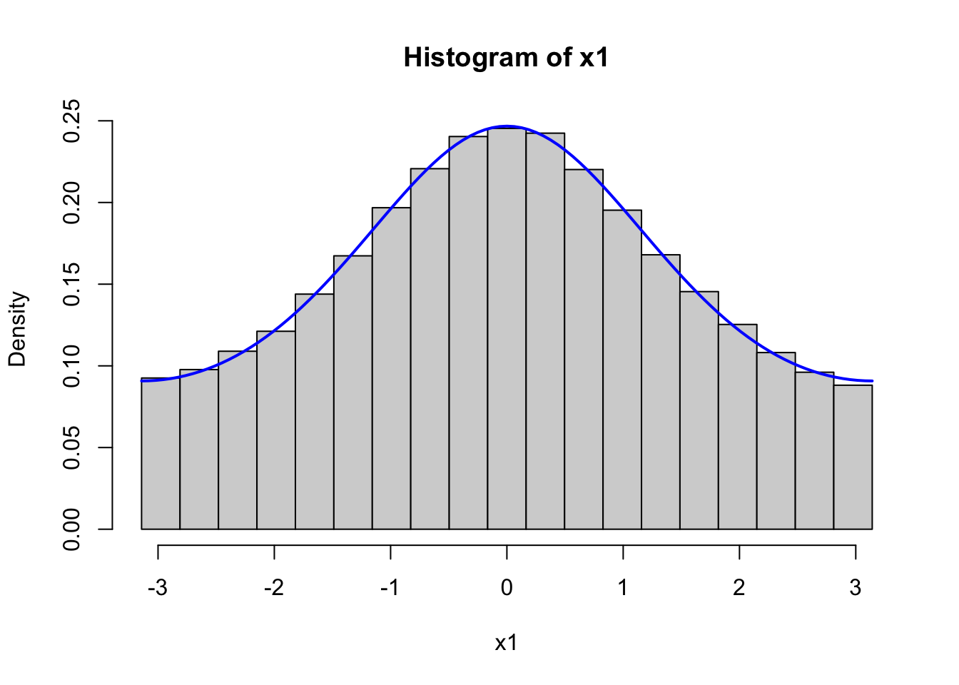
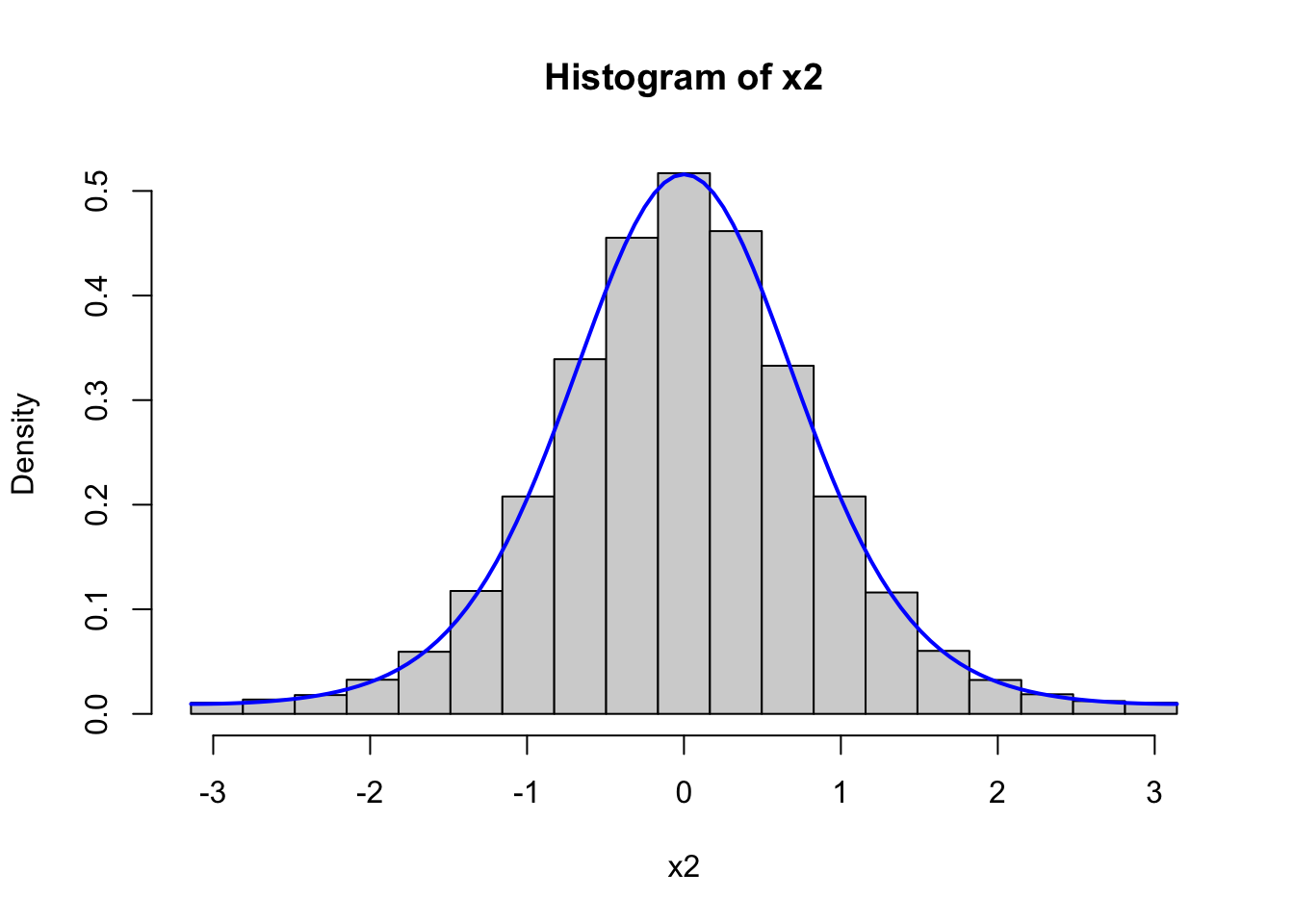
Figure 6.1: Histograms of 1,000 simulated data points from von Mises distributions with parameters \(\kappa = 0.5\) (left) and \(\kappa = 2\) (right). The true densities (blue) are added to the plots.
Figure 6.1 confirms that the implementation simulates from the von Mises distribution.
We then check how quickly the implementation can generate a large number of variables.
bench::system_time(von_mises_loop(100000, kappa = 5))## process real
## 598ms 589msThough the implementation can easily simulate 100,000 variables in less than two seconds, it might still be possible to improve it. To investigate what most of the runtime is spent on we use the line profiling tool as implemented in the profvis package, see also Section A.3.2.
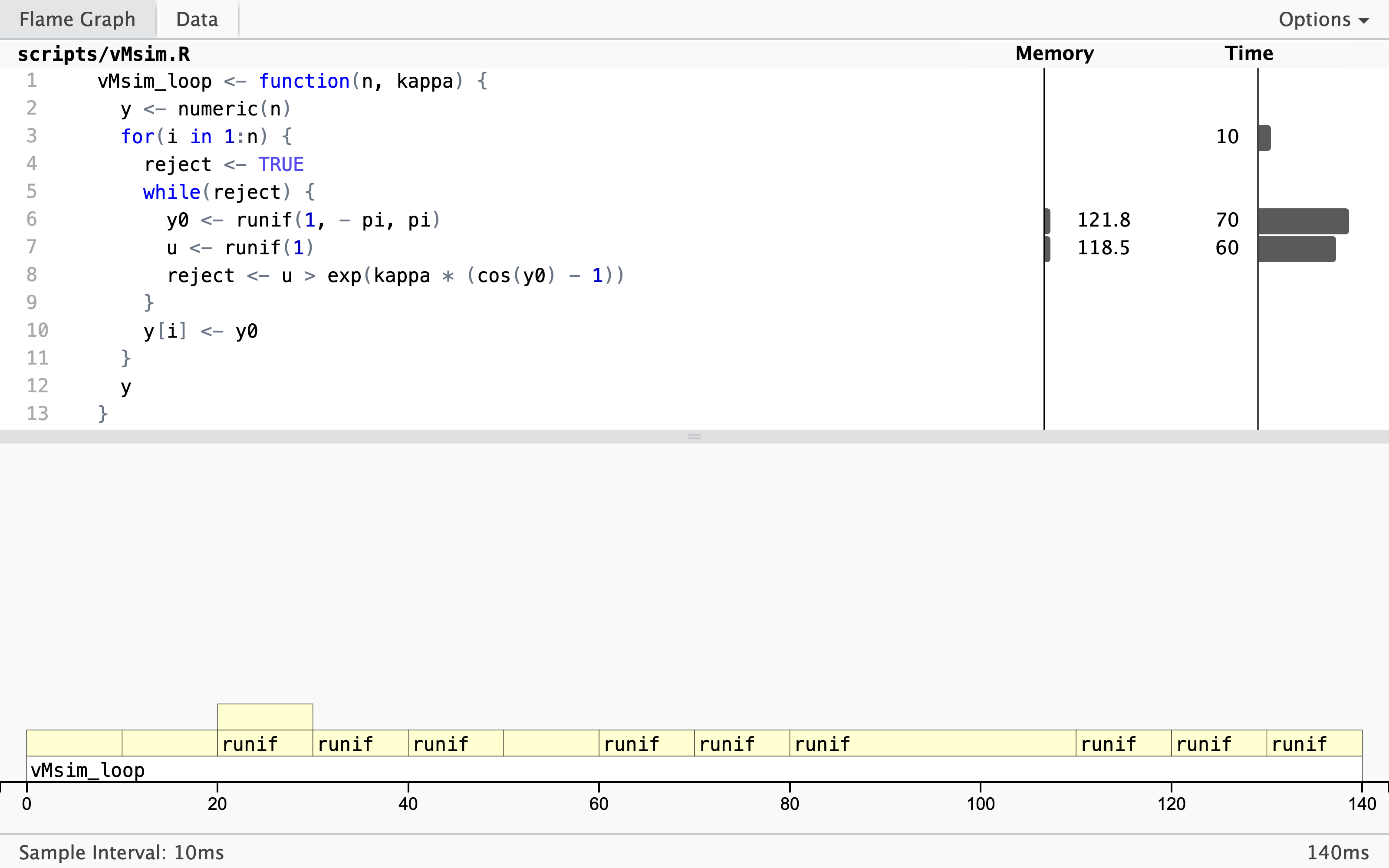
The profiling result shows that almost all the time
is spent on simulating uniformly distributed random variables. It is, perhaps,
expected that this should take some time, but that it takes so much more time
than computing the ratio, say, used for the rejection test is a bit surprising.
What might be even more surprising is the large amount of memory allocation
and deallocation associated with the simulation of the variables. The flame
graph above shows that this has also triggered calls to the the
garbage collector (the <GC> in the flame graph).
The culprit is runif() that has some overhead associated with each call.
The function performs much better if called once to return a vector than
if called repeatedly as above to return just single numbers. We could
rewrite the rejection sampler to make better use of runif(), but it would
make the code a bit more complicated because we do not know upfront
how many uniform variables we need. Sections A.2.3 and
A.3 in the appendix show how to implement caching via
a function factory to mitigate the inefficiency of generating random
numbers sequentially in R. We will not pursue that idea here but
instead focus on a fully vectorized implementation.
To write a runtime efficient R function we need to do more than just vectorize the generation of random numbers. We need to turn the entire rejection sampler into a vectorized computation. As all computations required are easily vectorized, it is straightforward to do so.
von_mises_random <- function(N, kappa) {
  x0 <- runif(N, - pi, pi)
  u <- runif(N)
  accept <- u <= exp(kappa * (cos(x0) - 1))
  x0[accept]
}
The only downside of the implementation above is that it returns a
random number of accepted samples instead of n samples. Since we do not
know upfront how many rejections there will be, there is no way around a
loop if we want to convert von_mises_random() into a function that returns
a fixed number of samples. We will need to solve this problem for
several other distributions, so we implement a general solution
that can convert any sampler generating a random number of samples into
a sampler that returns a fixed number of samples.
The solution is a function operator, much like Vectorize(),
that takes a function and returns a function.
The implementation below returns a sampler based on the function argument
rng. The sampler repeatedly calls rng() while adapting the number of proposals
after its first iteration by estimating the acceptance rate. The
two arguments fact and M_min control the adaptation with
defaults ensuring at least 100 proposals and otherwise 20% more
than estimated.
The implementation contains a few additional bells and whistles. First,
the ellipses argument, ..., is used, which captures all arguments to
a function and in this case passes them on via the call rng(M, ...).
Second, for the sake of subsequent usages in Section 6.2.3.
we include the callback argument cb, see also Section A.3.3.
rng_vec <- function(rng, fact = 1.2, M_min = 100) {
  CSwR::force_all()
  function(N, ..., cb) {
    j <- 0
    l <- 0     # The number of accepted samples
    x <- list()
    while (l < N) {
      j <- j + 1
      # Adapt the number of proposals
      M <- floor(max(fact * (N - l), M_min))
      x[[j]] <- rng(M, ...)
      l <- l + length(x[[j]])
      if (!missing(cb)) cb() # Callback
      # Update 'fact' by estimated acceptance probability l / n
      if (j == 1) fact <- fact * N / l
    }
    unlist(x)[1:N]
  }
}

von_mises_vec <- rng_vec(von_mises_random)
The implementation incrementally grows a list, whose entries contain vectors of accepted samples. It is usually not bad practice to dynamically grow objects (vectors or list), as this will result in unnecessary memory allocation, copying and deallocation. Thus it is better to initialize a vector of the correct size upfront. In this particular case the list will only contain relatively few entries, and it is inconsequential that it is grown dynamically.
Finally, a C++ implementation via Rcpp is given below where the random variables are then again generated one at a time via the C-interface to R’s random number generators. There is no (substantial) overhead of doing so in C++.
#include <Rcpp.h>
using namespace Rcpp;
// [[Rcpp::export]]
NumericVector von_mises_cpp(int N, double kappa) {
  NumericVector x(N);
  double x0;
  bool reject;
  for(int i = 0; i < N; ++i) {
    do {
      x0 = R::runif(- M_PI, M_PI);
      reject = R::runif(0, 1) > exp(kappa * (cos(x0) - 1));
    } while(reject);
    x[i] = x0;
  }
  return x;
}
We can test the vectorized implementation as well as the C++ implementation by comparing simulated variables to the theoretical distribution as above. Here we present instead a test of whether they produce variables from the same distribution via a QQ-plot. Figure 6.2 shows QQ-plots of variables simulated by the Rccp implementation against variables simulated by the vectorized R implementation. The points fall roughly on a straight line with slope 1 and intercept 0, which confirms that the implementations simulate from the same distribution.
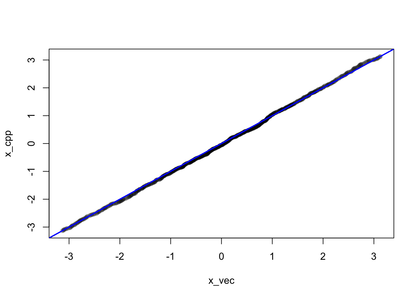
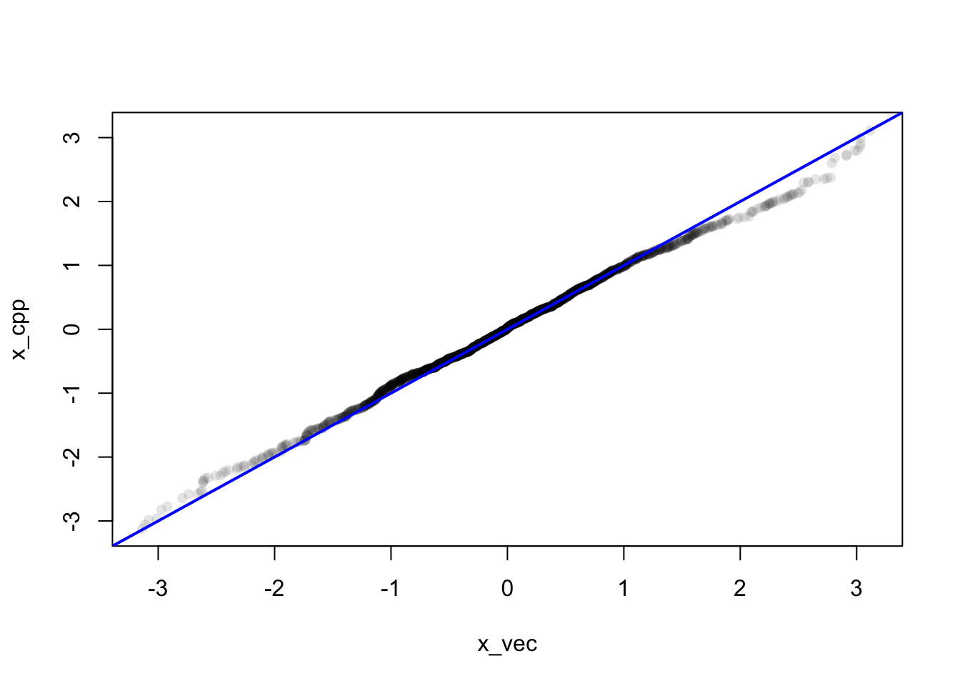
Figure 6.2: QQ-plots of 2,000 simulated data points from von Mises distributions with parameters \(\kappa = 0.5\) (left) and \(\kappa = 2\) (right), simulated using either the Rcpp implementation or the vectorized R implementation.
We conclude this section by measuring the runtime for all three implementations
of the von Mises rejection sampler using the mark() function from the bench package.
bench::mark(
  loop = von_mises_loop(1000, kappa = 5),
  vec = von_mises_vec(1000, kappa = 5),
  cpp = von_mises_cpp(1000, kappa = 5),
  check = FALSE,
  relative = TRUE
)
## # A tibble: 3 × 6
## expression min median `itr/sec` mem_alloc `gc/sec`
## <bch:expr> <dbl> <dbl> <dbl> <dbl> <dbl>
## 1 loop 43.6 36.1 1 1.32 Inf
## 2 vec 1 1 35.7 24.8 Inf
## 3 cpp 1.23 1.12 32.2 1 NaNThe C++ implementation and the vectorized R implementation have about
the same runtime, while the implementation in von_mises_loop(), using a for-loop in R,
is a factor 70 or so slower than the two others. Rejection sampling is a good example
of an algorithm for which a naive loop-based R implementation
performs rather poorly in terms of runtime, while a vectorized
implementation is competitive with an Rcpp implementation.
6.1.2 Rejection sampling from the gamma distribution
The gamma distribution with shape parameter \(r > 0\) has density
\[ f_r(x) = \frac{1}{\Gamma(r)} x^{r - 1} e^{-x}, \qquad x > 0. \]
It may be possible to find a suitable envelope of this density on \((0, \infty)\), but it turns out that there is a very efficient rejection sampler of a non-standard distribution that can be transformed into a gamma distribution by a simple transformation if \(r \geq 1\).
Let \(t(x) = a(1 + bx)^3\) for \(x \in (-b^{-1}, \infty)\). If \(r \geq 1\) and \(X\) has density
\[ f(x) \propto t(x)^{r-1}t'(x) e^{-t(x)} = e^{(r-1)\log t(x) + \log t'(x) - t(x)} \]
then \(t(X)\) is gamma distributed with shape parameter \(r \geq 1\) and density \(f_r\). The proof of this follows from a univariate change-of-variable, but see also the original paper by Marsaglia and Tsang (2000), who proposed the rejection sampler discussed in this section. The density \(f\) will be the target density for a rejection sampler using a standard Gaussian proposal distribution.
With
\[ f(x) \propto e^{(r-1)\log t(x) + \log t'(x) - t(x)}, \]
\(a = r - 1/3\) and \(b = 1/(3 \sqrt{a})\),
\[ f(x) \propto e^{a \log t(x)/a - t(x) + a \log a} \propto \underbrace{e^{a \log t(x)/a - t(x) + a}}_{q(x)}. \]
An analysis of \(w(x) := - x^2/2 - \log q(x)\) shows that it is convex on \((-b^{-1}, \infty)\) and it attains its minimum in \(0\) with \(w(0) = 0\), whence
\[ q(x) \leq e^{-x^2/2}. \]
This gives us an envelope expressed in terms of unnormalized densities with \(\alpha' = 1\).
The implementation of a rejection sampler based on this analysis is relatively
straightforward. The rejection sampler will simulate from the distribution
with density \(f\) by simulating from the Gaussian distribution (the envelope).
For the rejection step we need to implement \(q\). Finally, we also need
to implement \(t\) to transform the result from the rejection sampler to be
gamma distributed. The rejection sampler is otherwise implemented as for
the vectorized von Mises distribution except that we lower the argument
fact from its default value 1.2 to 1.1.
By doing so the initial batch of proposals will be 10% larger than the
desired sample size, and a second batch is rarely generated if the acceptance
rate is above 91%.
t_fun <- function(x, a) {
  b <- 1 / (3 * sqrt(a))
  (x > -1 / b) * a * (1 + b * x)^3  # 0 when y <= -1/b
}

q_fun <- function(x, r) {
  a <- r - 1 / 3
  t_val <- t_fun(x, a)
  exp(a * log(t_val / a) - t_val + a)
}

# Recall that the shape parameter has to fulfill: r >= 1
gamma_random <- function(N, r) {
  x0 <- rnorm(N)
  u <- runif(N)
  accept <- u <= q_fun(x0, r) * exp(x0^2 / 2)
  x <- x0[accept]
  t_fun(x, r - 1 / 3)
}

gamma_vec <- rng_vec(gamma_random, fact = 1.1)
We test the implementation by simulating \(100,000\) values with parameters \(r = 8\) as well as \(r = 1\) and compare the resulting histograms to the respective theoretical densities.
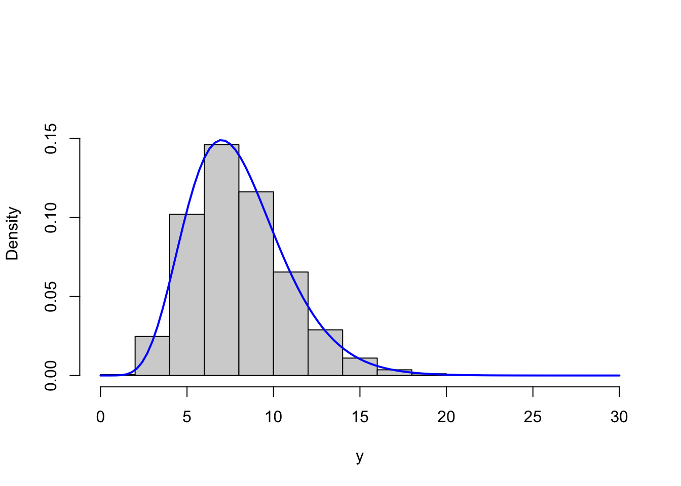
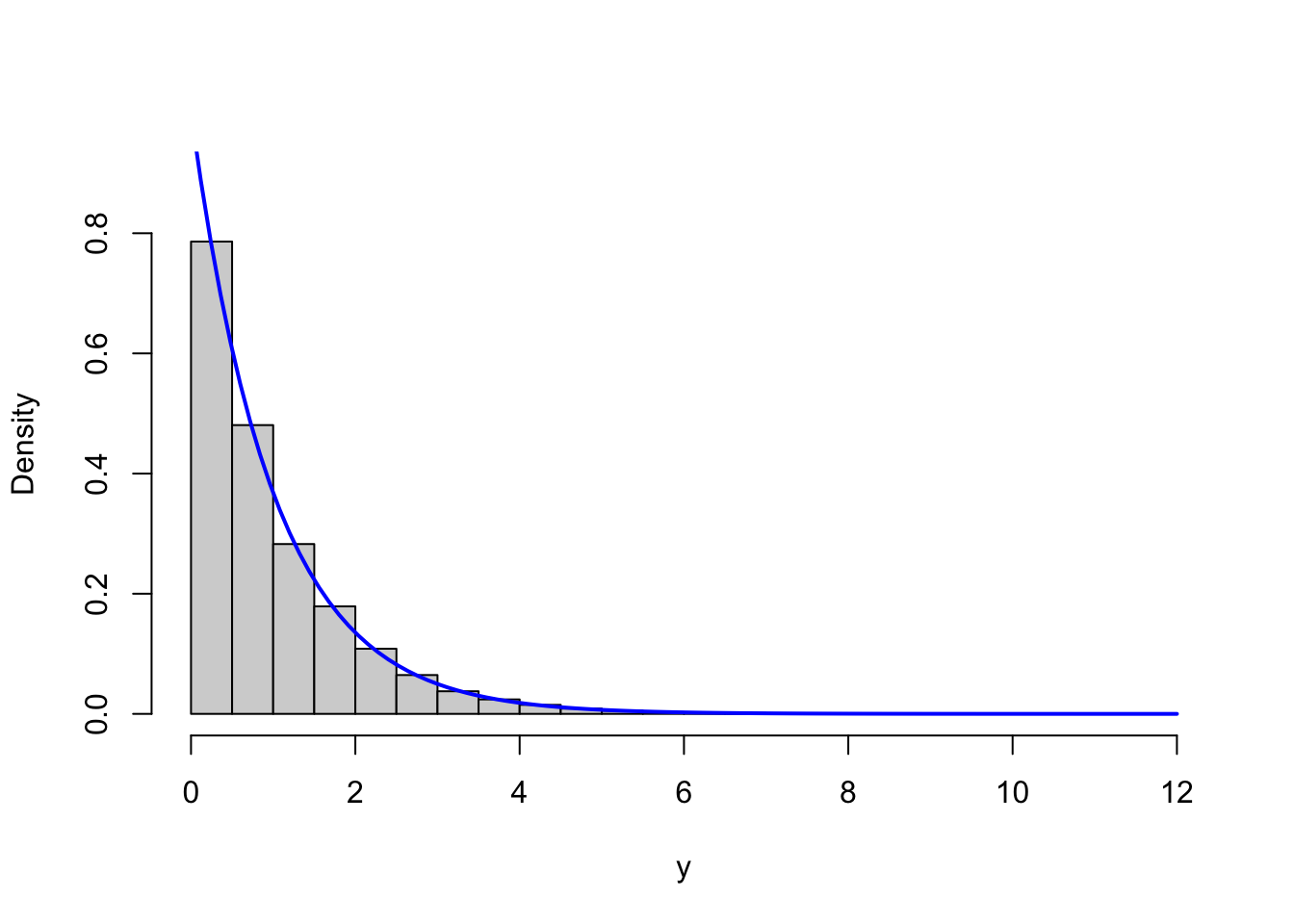
Figure 6.3: Histograms of simulated gamma distributed variables with shape parameters \(r = 8\) (left) and \(r = 1\) (right) with corresponding theoretical densities (blue).
This is a simple and informal test, but it does indicate that the implementation correctly simulates from the gamma distribution.
Rejection sampling can be computationally expensive if many samples are rejected. A very tight envelope will lead to fewer rejections, while a loose envelope will lead to many rejections. To investigate the acceptance rate we use the the callback argument with a tracer. The tracer computes an estimate of the acceptance rate from the first (and in most cases only) iteration in the loop.
gamma_tracer <- tracer(
  "alpha",
  # alpha is the estimated acceptance rate
  expr = quote(alpha <- l / M)
)
y <- gamma_vec(100000, 16, cb = gamma_tracer$trace)
y <- gamma_vec(100000, 8, cb = gamma_tracer$trace)
y <- gamma_vec(100000, 4, cb = gamma_tracer$trace)
y <- gamma_vec(100000, 1, cb = gamma_tracer$trace)
## n = 1: alpha = 0.9982;
## n = 2: alpha = 0.9963;
## n = 3: alpha = 0.9925;
## n = 4: alpha = 0.9527;We observe that the acceptance rates are large with \(r = 1\) being the worst case but still with more than 95% acceptances. For the larger values of \(r\), the acceptance rates are all above 99%, thus rejection is rare.
To better understand why rejection is rare for this rejection sampler, we can visually compare \(q\) to the unnormalized Gaussian density. Figure 6.4 does so for \(r = 1\) and \(r = 8\), and it shows that the Gaussian density is a very tight envelope—even for \(r = 1\). For \(r = 8\) we can only really see a difference between the target and the envelope on the log-density scale, and these differences are areas of the sample space where there is very little probability mass anyway.
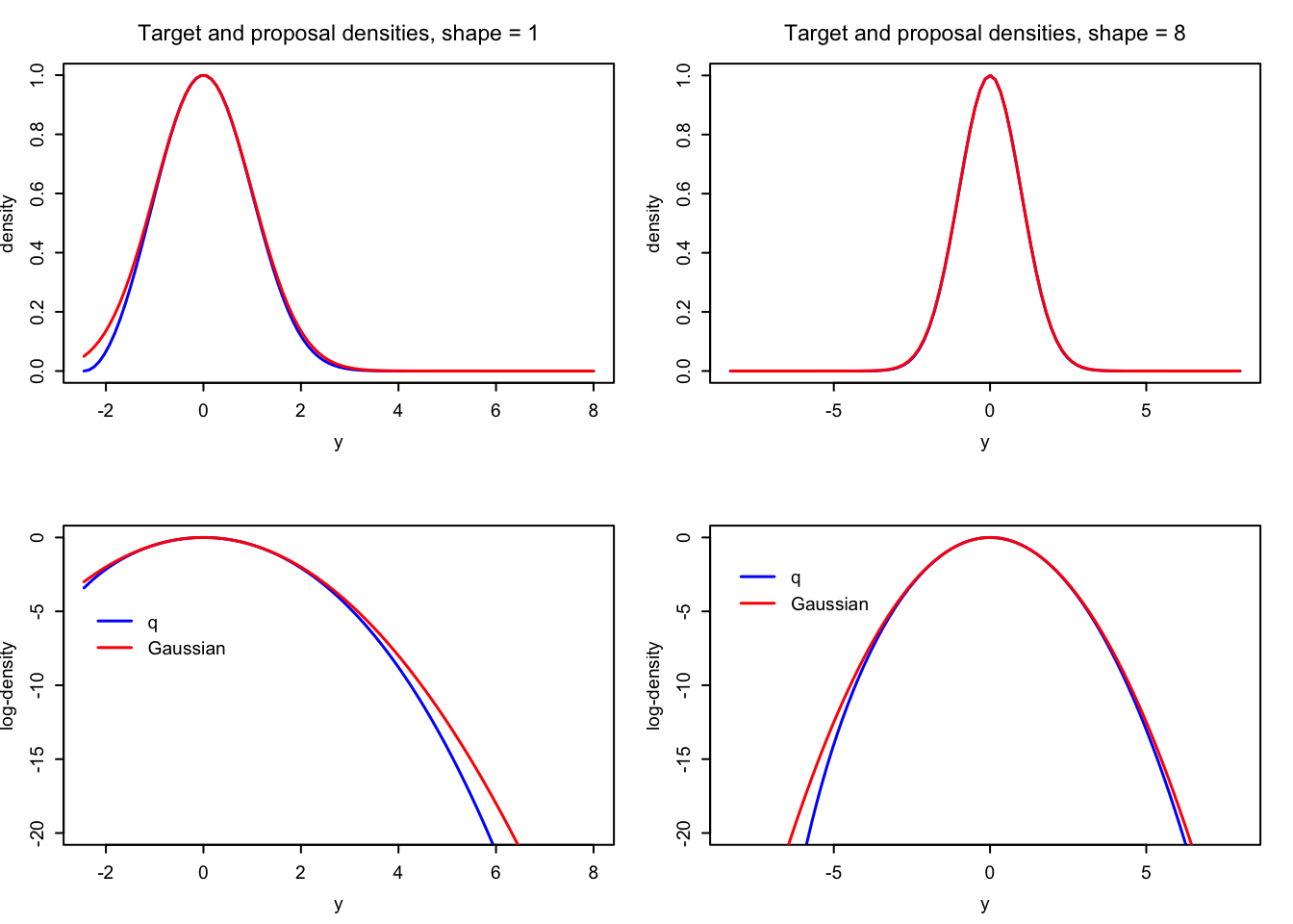
Figure 6.4: Comparisons of the Gaussian proposal (red) and the target density (blue) used for simulating gamma distributed variables via a transformation for two different values of the shape parameter.
6.2 Piecewise log-affine proposals
A good proposal should have \(\alpha\) close to one, it should be fast to simulate from and have a density that is fast to evaluate. It is not obvious how to find such an envelope for an arbitrary target density \(f\).
This section develops a general scheme for the construction of proposal distributions on \(\mathbb{R}\) with piecewise log-affine densities. The scheme is particularly useful for densities that are either log-concave or log-convex. The scheme leads to analytically manageable formulas for the envelope, its corresponding distribution function and its inverse, and as a result it is fast to simulate proposals from these distributions and evaluate the envelope as needed in the accept-reject step.
The proposal densities will be defined on an open interval \(I \subseteq \mathbb{R}\). Let
\[\begin{align*} I_1 & = (z_0, z_1] \\ I_2 &= (z_1, z_2] \\ & \vdots \\ I_m & = (z_{m-1}, z_m) \end{align*}\]
be non-empty subintervals of \(I\) forming a partition of \(I\). That is, we assume that \(I = (z_0, z_m)\) and that \(z_0 < z_1 < \ldots z_{m-1} < z_m\). Then endpoints \(z_0\) and \(z_m\) may be \(- \infty\) and \(+ \infty\), respectively. For \(a_i, b_i \in \mathbb{R}\) for \(i = 1, \ldots, m\) we define the piecewise affine function
\[ V(x) = \sum_{i=1}^m (a_i y + b_i) 1_{I_i}(x). \]
If
\[\begin{equation} d = \int_I e^{V(x)} \mathrm{d} x < \infty \tag{6.2} \end{equation}\]
then \(g(x) = d^{-1}e^{V(x)}\) is a density for a probability distribution on the interval \(I\), and this density is piecewise log-affine. The integrability condition (6.2) holds if and only if
- either \(0 < a_1\) and \(a_m < 0\)
- or \(0 < a_1\) and \(z_m < \infty\)
- or \(- \infty < z_0\) and \(a_m < 0\)
- or \(- \infty < z_0\) and \(z_m < \infty\).
The distribution function for such a probability distribution is given by
\[ G(x) = \frac{1}{d} \int_{z_0}^x e^{V(z)} \mathrm{d}z. \]
To simulate from a distribution with piecewise log-affine density, we can use Theorem 5.1 and transform uniformly distributed variables by the inverse distribution function. It requires a little bookkeeping, but is otherwise straightforward. Define for \(i = 1, \ldots, m\) the functions
\[ H_i(x) = \int_{z_{i-1}}^x e^{a_i z + b_i} \mathrm{d} z, \]
and let \(R_i = H_i(z_i)\) and \(Q_i = \sum_{k=1}^{i} R_k\). Then \(d = Q_m = \sum_{i=1}^m R_i\), and for \(q \in (0, 1)\), solving the equation \(G(x) = q\) is equivalent to solving the equation
\[\begin{equation} H_i(x) = dq - Q_{i-1} \tag{6.3} \end{equation}\]
if \(dq \in (Q_{i-1}, Q_{i}]\). That is, to compute \(G^{-1}(q)\) we first determine \(i\) such that \(Q_{i-1} < dq \leq Q_{i}\), and then we solve (6.3). To this end, note that for \(a_i \neq 0\),
\[ H_i(x) = \frac{1}{a_i}e^{b_i}\left(e^{a_i x} - e^{a_i z_{i-1}}\right). \]
Using proposal distributions with piecewise log-affine densities requires that we can verify the envelope condition, \(\alpha f \leq g\). We give an example where this condition follows from log-convexity of the target \(f\), and in Section 6.2.1 we give a systematic construction of envelopes for log-concave targets. Recall that we do not need to know the normalizing constant of \(f\), nor do we need to compute the normalizing constant \(d\) for the piecewise log-affine proposal.
Example 6.1 Consider the target density \(f(x) \propto e^{x^2}\) for \(x \in I = (0, 1)\). This density is log-convex since \(\log(e^{x^2}) = x^2\) is a convex function. For any \(u < w\) in \((0, 1)\) the chord connecting \((u, u^2)\) and \((w, w^2)\) is always above the graph of \(\log(e^{x^2})\) due to convexity. That is,
\[ e^{x^2} \leq e^{ax + b} \]
for \(y \in [u, w]\) if \(a\) and \(b\) are chosen so that \(au + b = u^2\) and \(aw + b = w^2\).
Taking \(z_0 = 0\) and \(z_1 = 1\), it follows that a piecewise log-affine bound over all of \(I = (0, 1)\) using the corresponding chord becomes
\[ e^{x^2} \leq e^{x} \]
for \(y \in (0, 1)\).
Taking \(z_0 = 0\), \(z_1 = 1/2\) and \(z_2 = 1\) a piecewise log-affine bound using the chords for each of the intervals \((0, 1/2]\) and \((1/2, 1)\) becomes
\[ e^{x^2} \leq e^{(x/2)1_{(0, 1/2]}(x) + (3x/2 - 1/2) 1_{(1/2, 1)}(x)}. \]
This leads to a tighter envelope than using the bound \(e^{x}\). By increasing the number of \(z\)-s we can make this envelope as tight as we want. This will lower the rejection probability but also increase the complexity of simulating from the proposal.
6.2.1 Log-concave densities
In this section we give a systematic construction of piecewise log-affine proposal densities for log-concave target densities, which form a relatively large class of unimodal densities.
We suppose that \(f : I \to (0, \infty)\) is (proportional to) a continuously differentiable, strictly positive and log-concave target density on the open interval \(I \subseteq \mathbb{R}\). For any partition \(I_1, \ldots, I_m \subseteq I\) as above and any collection of points \(y_1 < y_2 < \ldots < y_{m}\) with \(y_i \in I_i\) we define
\[ a_i = (\log(f(x_i)))' = \frac{f'(x_i)}{f(x_i)} \quad \text{and} \quad b_i = \log(f(x_i)) - \alpha_i x_i \]
By log-concavity,
\[ \log(f(x)) \leq \frac{f'(x_i)}{f(x_i)}(x - y_i) + \log(f(x_i)) = a_ix + b_i \]
for \(y \in I\). Thus
\[ \log(f(x)) \leq V(x) = \sum_{i=1}^m (a_i x + b_i) 1_{I_i}(x), \]
or
\[ f(x) \leq e^{V(x)}. \]
Provided that the integrability condition (6.2) holds, the piecewise log-affine density proportional to \(e^{V(x)}\) can then be used as proposal density for rejection sampling from \(f\) with \(\alpha' = 1\).
The bounds are constructed so that \(f(x_i) = e^{V(x_i)}\) for \(i = 1, \ldots, m\), thus the envelope touches the target density and we cannot increase \(\alpha'\) beyond \(1\). We can, however, tighten the envelope by adapting the boundary points \(z_1, \ldots, z_{m-1}\) of the \(I_i\)-intervals to the points \(y_1, \ldots, y_m\). The rejection probability is minimized if \(a_i x + b_i\) is minimal over \(I_i\) among all the affine upper bounds. By the log-concavity, \(a_1 \geq a_2 \geq \ldots \geq a_m\), and for \(a_{i+1} < a_i\) we can choose
\[ z_i = \frac{b_{i+1} - b_i}{a_i - a_{i+1}} \]
for \(i = 1, \ldots, m - 1\). Then \(z_i\) is the solution to the equation \(a_i x + b_i = a_{i+1} x + b_{i+1}\), and it is the point where the two corresponding tangents to the graph of \(\log(f)\) intersect.
For log-concave densities, the contructions above give us, for any fixed collection of points \(y_1 < \ldots < y_m\) in \(I\), a tight piecewise log-affine envelope. It is obtained by first computing the \(a_i\)-s and \(b_i\)-s and then the \(z_i\)-s.
For some applications, notably when simulating from a posterior distribution for a large dataset within a Bayesian model framework, the target density \(f\) might be expensive to evaluate. If \(f\) is log-concave, we can also bound it from below by a piecewise log-affine function, but using chords instead of tangents, similarly to the construction in Example 6.1. Such a lower bound, which is cheap to evaluate, could make the accept-reject step faster. It is also possible to choose the points \(y_1 < \ldots < y_m\) automatically and by an adaptive algorithm. We will not pursue such potential improvements and generalizations, see (Gilks and Wild 1992) for details.
6.2.2 Beta distribution
To illustrate the envelope construction above for a simple log-concave density we consider the beta distribution on \((0, 1)\) with shape parameters \(\geq 1\). This distribution has density \[f(x) \propto x^{\alpha - 1}(1-x)^{\beta - 1},\] which is log-concave (when both shape parameters are greater than one). We implement the rejection sampling algorithm for this density with the piecewise log-affine envelope having two pieces—determined by two user-supplied points.
beta_random <- function(N, x1, x2, alpha, beta) {
  lf <- function(x) (alpha - 1) * log(x) + (beta - 1) * log(1 - x)
  lf_deriv <- function(x) (alpha - 1) / x - (beta - 1) / (1 - x)
  a1 <- lf_deriv(x1)
  a2 <- lf_deriv(x2)
  if (a1 == 0 || a2 == 0 || a1 - a2 == 0)
    stop("\n
    The implementation requires a1 and a2 different and both different
    from zero. Choose different values of x1 and x2 to ensure this."
    )
  b1 <- lf(x1) - a1 * x1
  b2 <- lf(x2) - a2 * x2
  z1 <- (b2 - b1) / (a1 - a2)
  Q1 <- exp(b1) * (exp(a1 * z1) - 1) / a1
  c <- Q1 + exp(b2) * (exp(a2 * 1) - exp(a2 * z1)) / a2

  x <- numeric(N)
  accept <- logical(N)
  u0 <- c * runif(N)
  u <- runif(N)

  I <- u0 < Q1
  x[I] <- log(a1 * exp(-b1) * u0[I] + 1) / a1
  accept[I] <- u[I] <= exp(lf(x[I]) - a1 * x[I] - b1)
  x[!I] <- log(a2 * exp(-b2) * (u0[!I] - Q1) + exp(a2 * z1)) / a2
  accept[!I] <- u[!I] <= exp(lf(x[!I]) - a2 * x[!I] - b2)

  x[accept]
}

beta_vec <- rng_vec(beta_random)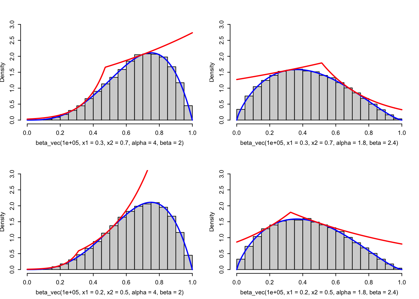
Figure 6.5: Histograms of simulated variables from beta distributions using the rejection sampler with the adaptive envelope based on log-concavity. The true density (blue) and the envelope (red) are added to the plots.
Note that as a safeguard we implemented a test on the \(a_i\)-s to check that the formulas used are actually meaningful, specifically that there are no divisions by zero.
beta_vec(1, x1 = 0.25, x2 = 0.75, alpha = 4, beta = 2)## Error in rng(M, ...):
##
## The implementation requires a1 and a2 different and both different
## from zero. Choose different values of x1 and x2 to ensure this.
beta_vec(1, x1 = 0.2, x2 = 0.75, alpha = 4, beta = 2)## Error in rng(M, ...):
##
## The implementation requires a1 and a2 different and both different
## from zero. Choose different values of x1 and x2 to ensure this.
beta_vec(1, x1 = 0.2, x2 = 0.8, alpha = 4, beta = 2)## [1] 0.79226.2.3 von Mises distribution
The von Mises rejection sampler in Section 6.1.1 used the uniform distribution as proposal distribution. As it turns out, the uniform density is not a particularly tight envelope. We illustrate this by studying the acceptance rate for our previous implementation.
von_mises_tracer <- tracer(
  c("r", "l", "MM"),
  N = 0,
  time = FALSE,
  expr = quote({
    r <- ..1
    if (j == 1) MM <- M else MM <- MM + M
  }
  )
)
y <- von_mises_vec(10000, 0.1, cb = von_mises_tracer$trace)
y <- von_mises_vec(10000, 0.5, cb = von_mises_tracer$trace)
y <- von_mises_vec(10000, 2, cb = von_mises_tracer$trace)
y <- von_mises_vec(10000, 5, cb = von_mises_tracer$trace)
## n = 1: l = 10907; r = 0.1; MM = 12000;
## n = 2: l = 7727; r = 0.5; MM = 12000;
## n = 3: l = 10013; r = 0.5; MM = 15529;
## n = 4: l = 3683; r = 2; MM = 12000;
## n = 5: l = 10007; r = 2; MM = 32582;
## n = 6: l = 2238; r = 5; MM = 12000;
## n = 7: l = 9809; r = 5; MM = 53619;
## n = 8: l = 10017; r = 5; MM = 54643;
trace_sum <- summary(von_mises_tracer)
trace_sum$alpha <- trace_sum$l / trace_sum$MM
trace_sum[trace_sum$l >= 10000, ]
## l r MM alpha
## 1 10907 0.1 12000 0.9089
## 3 10013 0.5 15529 0.6448
## 5 10007 2.0 32582 0.3071
## 8 10017 5.0 54643 0.1833The acceptance rate decreases with \(\kappa\) and is fairly small unless \(\kappa\) is small. For \(\kappa = 5\) less than 20% of the proposals are accepted, and simulating \(n = 10,000\) von Mises distributed variables thus requires the simulation of more than \(50,000\) variables from the proposal.
The von Mises density is, unfortunately, not log-concave on \((-\pi, \pi)\), but it is on \((-\pi/2, \pi/2)\). It is, furthermore, log-convex on \((-\pi, -\pi/2)\) as well as \((\pi/2, \pi)\), which implies that on these two intervals the log-density is below the corresponding chords. These chords can be pieced together with tangents to give an envelope. We first implement the algorithm that returns a random length vector.
von_mises_adapt_random <- function(N, x1, x2, kappa) {
  lf <- function(x) kappa * cos(x)
  lf_deriv <- function(x) - kappa * sin(x)
  a1 <- 2 * kappa / pi
  a2 <- lf_deriv(x1)
  a3 <- lf_deriv(x2)
  a4 <- - a1

  b1 <- kappa
  b2 <- lf(x1) - a2 * x1
  b3 <- lf(x2) - a3 * x2
  b4 <- kappa

  z0 <- -pi
  z1 <- -pi / 2
  z2 <- (b3 - b2) / (a2 - a3)
  z3 <- pi / 2
  z4 <- pi

  Q1 <- exp(b1) * (exp(a1 * z1) - exp(a1 * z0)) / a1
  Q2 <- Q1 + exp(b2) * (exp(a2 * z2) - exp(a2 * z1)) / a2
  Q3 <- Q2 + exp(b3) * (exp(a3 * z3) - exp(a3 * z2)) / a3
  c <- Q3 + exp(b4) * (exp(a4 * z4) - exp(a4 * z3)) / a4

  u0 <- c * runif(N)
  u <- runif(N)

  I1 <- (u0 < Q1)
  I2 <- (u0 >= Q1) & (u0 < Q2)
  I3 <- (u0 >= Q2) & (u0 < Q3)
  I4 <- (u0 >= Q3)

  x <- numeric(N)
  accept <- logical(N)
  x[I1] <- log(a1 * exp(-b1) * u0[I1] + exp(a1 * z0)) / a1
  accept[I1] <- u[I1] <= exp(lf(x[I1]) - a1 * x[I1] - b1)
  x[I2] <- log(a2 * exp(-b2) * (u0[I2] - Q1) + exp(a2 * z1)) / a2
  accept[I2] <- u[I2] <= exp(lf(x[I2]) - a2 * x[I2] - b2)
  x[I3] <- log(a3 * exp(-b3) * (u0[I3] - Q2) + exp(a3 * z2)) / a3
  accept[I3] <- u[I3] <= exp(lf(x[I3]) - a3 * x[I3] - b3)
  x[I4] <- log(a4 * exp(-b4) * (u0[I4] - Q3) + exp(a4 * z3)) / a4
  accept[I4] <- u[I4] <=  exp(lf(x[I4]) - a4 * x[I4] - b4)

  x[accept]
}
Then we turn the implementation into a function that returns a fixed number of samples, and using the tracer we estimate the acceptance rates for four different combinations of parameters and partition points.
von_mises_adapt <- rng_vec(von_mises_adapt_random)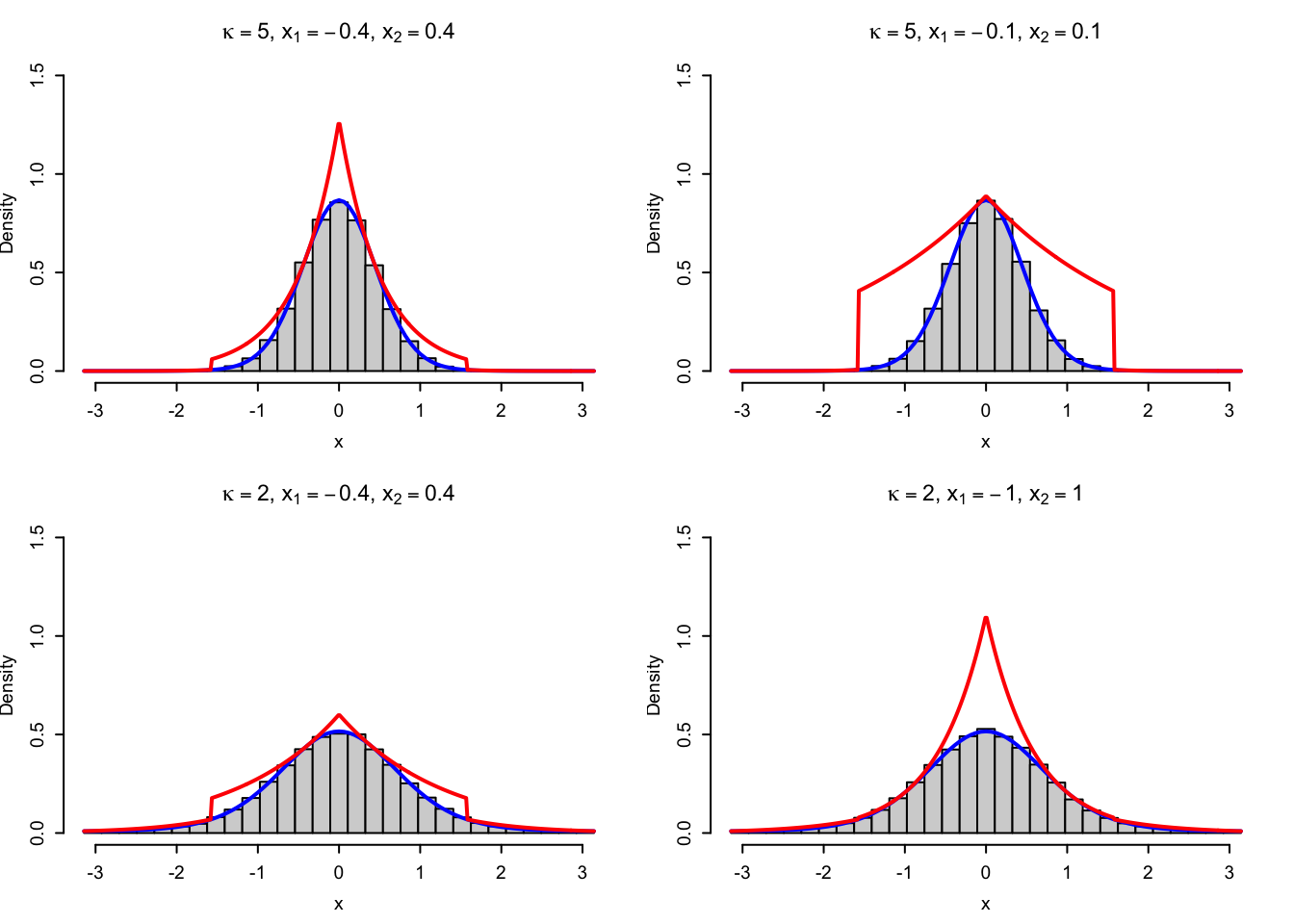
Figure 6.6: Histograms of simulated variables from von Mises distributions using the rejection sampler with the adaptive envelope based on a combination of log-concavity and log-convexity. The true density (blue) and the envelope (red) are added to the plots.
von_mises_tracer$clear()
y <- von_mises_adapt(10000, -0.4, 0.4, 5, cb = von_mises_tracer$trace)
y <- von_mises_adapt(10000, -0.1, 0.1, 5, cb = von_mises_tracer$trace)
y <- von_mises_adapt(10000, -0.4, 0.4, 2, cb = von_mises_tracer$trace)
y <- von_mises_adapt(10000, -1, 1, 2, cb = von_mises_tracer$trace)
## n = 1: l = 9602; r = -0.4; MM = 12000;
## n = 2: l = 10001; r = -0.4; MM = 12497;
## n = 3: l = 6224; r = -0.1; MM = 12000;
## n = 4: l = 10020; r = -0.1; MM = 19280;
## n = 5: l = 10098; r = -0.4; MM = 12000;
## n = 6: l = 9130; r = -1; MM = 12000;
## n = 7: l = 9997; r = -1; MM = 13143;
## n = 8: l = 10075; r = -1; MM = 13243;
## l r MM alpha
## 2 10001 -0.4 12497 0.8003
## 4 10020 -0.1 19280 0.5197
## 5 10098 -0.4 12000 0.8415
## 8 10075 -1.0 13243 0.7608We see that compared to using the uniform density as envelope, these adaptive envelopes are generally tighter and leads to fewer rejections. Even tighter envelopes are possible by using more than four intervals, but it is, of course, always a good question how the added complexity and bookkeeping induced by using more advanced and adaptive envelopes affect runtime. It is even a good question if our current adaptive implementation will outperform our much simpler implementation that used the uniform envelope.
bench::mark(
  adapt1 = von_mises_adapt(100, -1, 1, 5),
  adapt2 = von_mises_adapt(100, -0.4, 0.4, 5),
  adapt3 = von_mises_adapt(100, -0.2, 0.2, 5),
  adapt4 = von_mises_adapt(100, -0.1, 0.1, 5),
  vec = von_mises_vec(100, 5),
  check = FALSE
)
## # A tibble: 5 × 6
## expression min median `itr/sec` mem_alloc `gc/sec`
## <bch:expr> <bch:tm> <bch:tm> <dbl> <bch:byt> <dbl>
## 1 adapt1 44.6µs 66.5µs 14991. 68.8KB 7.50
## 2 adapt2 22.9µs 48.1µs 21789. 59.9KB 7.74
## 3 adapt3 41µs 47.9µs 20083. 59.8KB 7.68
## 4 adapt4 41µs 49.1µs 19483. 59.1KB 7.83
## 5 vec 16.4µs 23.9µs 40532. 25.1KB 4.05The results from the benchmark show that the adaptive implementation has runtime comparable to but slightly slower than using the uniform proposal. With \(x_1 = -0.4\) and \(x_2 = 0.4\) and \(\kappa = 5\) we found above that the acceptance rate was about 80% with the adaptive envelope, while it was below 20% when using the uniform envelope. A naive computation would thus suggest a speedup of a factor 4, but using the adaptive envelope there is actually no speedup with the current implementation. It is left as an exercise to implement the adaptive rejection sampler in Rcpp to test if any speedup can be obtained in this way.
The benchmarks above show that when comparing algorithms and their implementations we should not get too focused on surrogate performance quantities. The acceptance rate is a surrogate for actual runtime. It might in principle be of interest to increase this probability, but if it is at the expense of additional computations it might not be worth the effort in terms of actual runtime.
6.3 Exercises
Exercise 6.1 Implement rejection sampling from the standard Gaussian distribution with density
\[ f(x) = \frac{1}{\sqrt{2\pi}} e^{- x^2 / 2} \]
by simulating Laplace random variables as proposals (see Exercises 5.3 and 5.4). Test the implementation by computing the empirical mean and variance of the simulated variables and compare with those of the Gaussian distribution. Compare also directly with the Gaussian distribution using histograms and QQ-plots.
Note: The Laplace distribution can be seen as a simple version of the piecewise log-affine envelopes treated in Section 6.2.