12 The stochastic EM algorithm
This chapter treats a single larger example that requires a combination of several of the computational methods covered in the book. The example is based on a stochastic volatility model, which is a time series model used in financial econometrics. The overall objective is to simultaneously estimate the parameters of the time series model and predict a latent component of the model.
Since the model specification contains and unobserved component, the EM algorithm is a natural candidate for parameter estimation. The computation of the conditional expectation, required by the EM algorithm, is, however, intractable, and we will therefore replace this computation by samples from an approximating conditional distribution. The result is a stochastic EM algorithm, which can be seen as an example of a stochastic optimization algorithm.
12.1 The stochastic volatility model
The stochastic volatility models is a bivariate time series model of \((Y_1, Z_1), \ldots, (Y_N, Z_N)\) given by the following equations for \(i = 1, \ldots, N\):
\[\begin{align} Z_{i} &= \mu + \alpha (Z_{i-1} - \mu) + \tau \varepsilon_i \tag{12.1} \\ Y_{i} &= \beta \exp(Z_{i} / 2) \eta_i \tag{12.2} \end{align}\]
where \(\varepsilon_1, \ldots, \varepsilon_N\) and \(\eta_1, \ldots, \eta_N\) are independent standard normal random variables, and where \(Z_0 = \mu\) by convention. The four model parameters are \(\beta, \mu, \alpha \in \mathbb{R}\) and \(\tau > 0\). We usually assume that \(|\alpha| < 1\) to ensure that the model is asymptotically stable.
Only the time series \((Y_1, \ldots, Y_N)\) is observed, and the goal is to estimate the parameters \(\beta, \mu, \alpha\) and \(\tau\). Since the \(Z\)-variables are unobserved, the likelihood function is intractable,
12.2 Data simulation
sv_sim <- function(N, par) {
  beta <- par["beta"]
  mu <- par["mu"]
  phi <- par["phi"]
  tau <- par["tau"]
  Z <- numeric(N)
  epsilon <- rnorm(N, sd = tau)
  Z[1] <- mu
  for (i in 2:N) {
    Z[i] <- mu + phi * (Z[i-1] - mu) + epsilon[i]
  }
  Y <- rnorm(N, sd = beta * exp(Z / 2))
  data.frame(Y = Y, Z = Z)
}
set.seed(124)
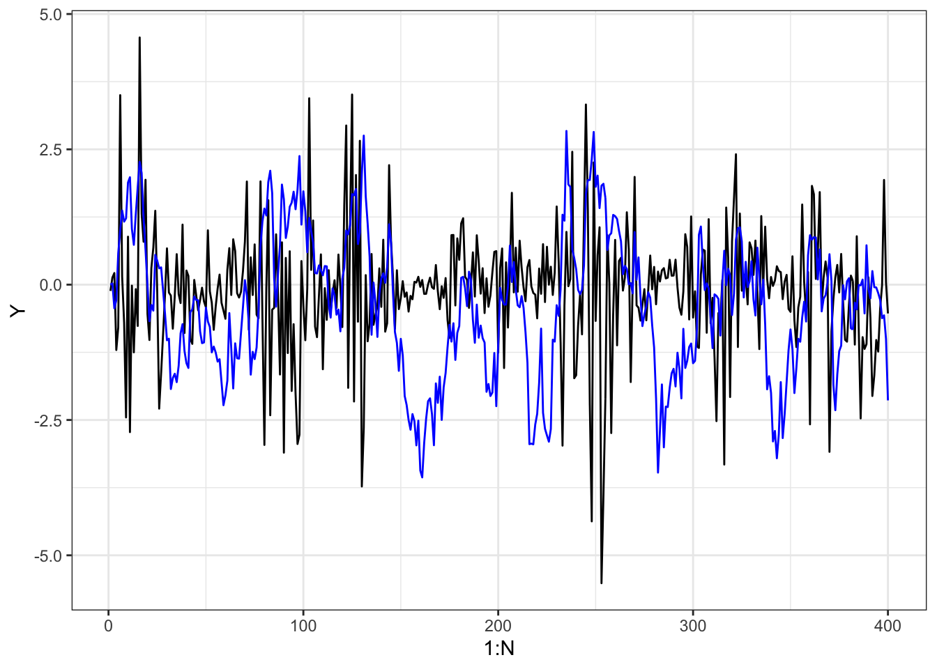
N <- 400
par <- c(beta = 1, mu = 0, phi = 0.95, tau = 0.6)
sv_tmp <- sv_sim(N, par)
ggplot(sv_tmp, aes(x = 1:N, y = Y)) +
geom_line() +
geom_line(aes(y = Z), color = "blue")