4 Time series smoothing
- Spatial / temporal data
- Stationarity / non-stationarity
- Sometimes called filtering (causal filters)
X variable fixed
p_Nuuk <- ggplot(nuuk, aes(x = Year, y = Temperature)) +
geom_line(color = "gray") + geom_point()
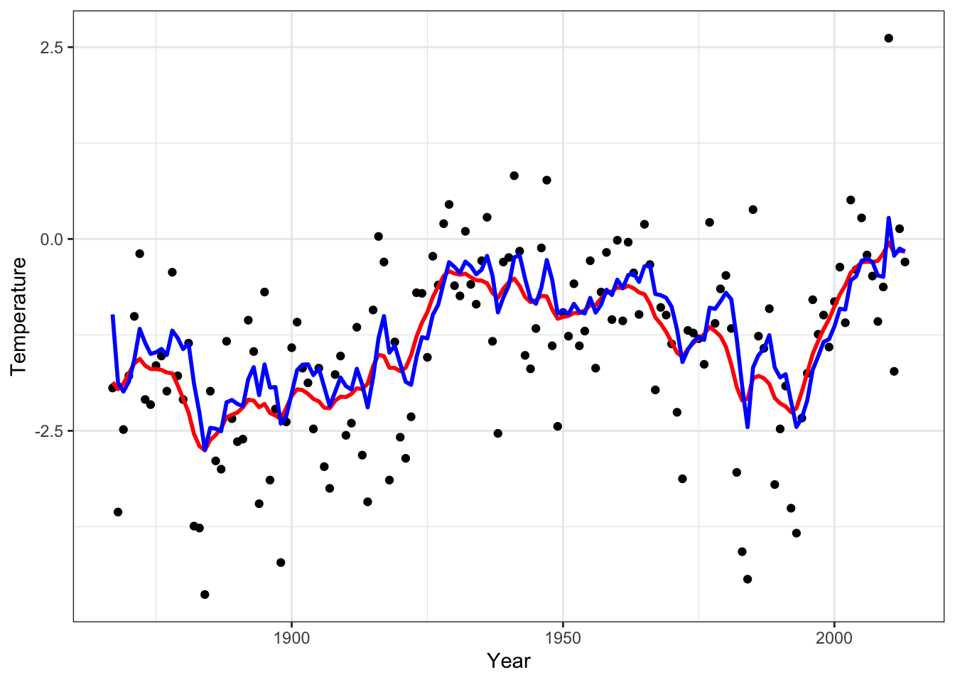
p_Nuuk +
geom_line(
aes(y = stats::filter(Temperature, rep(1/21, 21))),
color = "blue", lwd = 1
)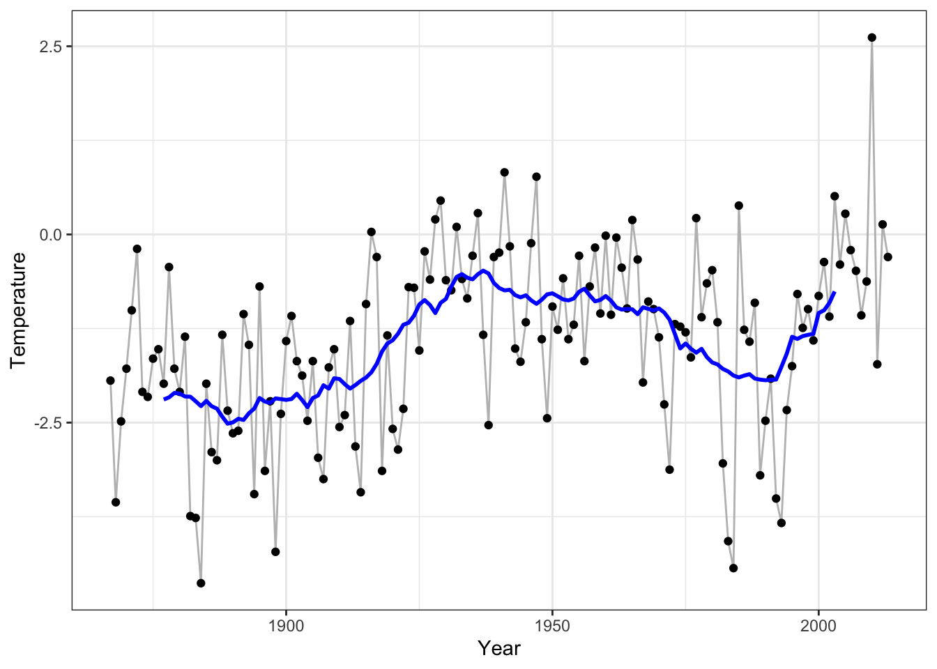
Figure 4.1: The time series of the annual average temperature in degrees Celsius in Nuuk from 1867 to 2013, smoothed using a simple running mean with a window size of 21 (blue).
4.1 Running mean
In this chapter we focus mostly on \(x\) being real valued with the ordinary metric used to define the nearest neighbors. The total ordering of the real line adds a couple of extra possibilities to the definition of \(\mathcal{N}_i\). When \(k\) is odd, the symmetric nearest neighbor smoother takes \(\mathcal{N}_i\) to consist of \(x_i\) together with the \((k-1)/2\) smaller \(x_j\)-s closest to \(x_i\) and the \((k-1)/2\) larger \(x_j\)-s closest to \(x_i\). It is also possible to choose a one-sided smoother with \(\mathcal{N}_i\) corresponding to the \(k\) smaller \(x_j\)-s closest to \(x_i\), in which case the smoother would be known as a causal filter.
The symmetric definition of neighbors makes it very easy to handle the neighbors computationally; we don’t need to compute and keep track of the \(n^2\) pairwise distances between the \(x_i\)-s, we only need to sort data according to the \(x\)-values. Once data is sorted,
\[ \mathcal{N}_i = \{i - (k - 1) / 2, i - (k - 1) / 2 + 1, \ldots, i - 1 , i, i + 1, \ldots, i + (k - 1) / 2\} \]
for \((k - 1) / 2 \leq i \leq N - (k - 1) / 2\). The symmetric \(k\) nearest neighbor smoother is thus a running mean of the \(y\)-values when sorted according to the \(x\)-values. There are a couple of possibilities for handling the boundaries, one being simply to not define a value of \(\hat{f}_i\) outside of the interval above.
With \(\hat{\mathbf{f}}\) denoting the vector of smoothed values by a nearest neighbor smoother we can observe that it is always possible to write \(\hat{\mathbf{f}} = \mathbf{S}\mathbf{y}\) for a matrix \(\mathbf{S}\). For the symmetric nearest neighbor smoother and with data sorted according to the \(x\)-values, the matrix has the following band diagonal form
\[ \mathbf{S} = \left( \begin{array}{cccccccccc} \frac{1}{5} & \frac{1}{5} & \frac{1}{5} & \frac{1}{5} & \frac{1}{5} & 0 & 0 & \ldots & 0 & 0 \\ 0 & \frac{1}{5} & \frac{1}{5} & \frac{1}{5} & \frac{1}{5} & \frac{1}{5} & 0 & \ldots & 0 & 0\\ 0 & 0 & \frac{1}{5} & \frac{1}{5} & \frac{1}{5} & \frac{1}{5} & \frac{1}{5} & \ldots & 0 & 0 \\ \vdots & \vdots & \vdots & \vdots & \vdots & \vdots & \vdots & \ldots & \vdots & \vdots \\ 0 & 0 & 0 & 0 & 0 & 0 & 0 & \ldots & \frac{1}{5} & \frac{1}{5} \\ \end{array} \right) \]
here given for \(k = 5\) and with dimensions \((N - 4) \times N\) due to the undefined boundary values.
4.1.1 Linear smoothers
A smoother of the form \(\hat{\mathbf{f}} = \mathbf{S}\mathbf{y}\) for a smoother matrix \(\mathbf{S}\), such as the nearest neighbor smoother, is known as a linear smoother. The linear form is often beneficial for theoretical arguments, and many smoothers considered in this chapter will be linear smoothers. For computing \(\mathbf{f}\) there may, however, be many alternatives to forming the matrix \(\mathbf{S}\) and computing the matrix-vector product. Indeed, this is often not the best way to compute the smoothed values.
It is, on the other hand, useful to see how \(\mathbf{S}\) can be constructed for the symmetric nearest neighbor smoother.
## Warning in matrix(w, 147 - 10, 147, byrow = TRUE): data length [148] is not a
## sub-multiple or multiple of the number of rows [137]
The construction above relies on vector recycling of w in the construction of S
and the fact that w has length \(147 + 1\), which will effectively cause w to be
translated by one to the right every time it is recycled for a new row. As seen,
the code triggers a warning by R, but in this case we get what we want.

Figure 4.2: Visualization of the smoother matrix \(S\). The gray diagonal band represents the non-zero entries.
run_mean_smoother <- function(N, k) {
  # truncate k to nearest odd integer
  m <- floor((k - 1) / 2)
  k <- 2 * m + 1
  w <- c(rep(1 / k, k), rep(0, N - k + 1))
  S <- matrix(NA, N, N)
  S[(m + 1):(N - m), ] <- suppressWarnings(
    matrix(w, N - k + 1, N, byrow = TRUE)
  )
  S
}
We can use the matrix to smooth the annual average temperature in Nuuk using a
running mean with a window of \(k = 11\) years. That is, the smoothed temperature
at a given year is the average of the temperatures in the period
from five years before to five years after. Note that to add the smoothed
values to the previous plot we need to pad the values at the boundaries
with NAs to get a vector of length 147.
# Check first if data is sorted correctly.
# The test is backwards, but confirms that data isn't unsorted :-)
is.unsorted(nuuk$Year)
## [1] FALSE
f_hat <- run_mean_smoother(147, 11) %*% nuuk$Temperature
p_Nuuk + geom_line(aes(y = f_hat), color = "blue")
Figure 4.3: Annual average temperature in Nuuk smoothed using the running mean with \(k = 11\) neighbors.
4.1.2 Implementing the running mean
The running mean smoother fulfills the following identity
\[ \hat{f}_{i+1} = \hat{f}_{i} - y_{i - (k-1)/2} / k + y_{i + (k + 1)/2} / k, \]
which can be used for a much more efficient implementation than the matrix-vector multiplication. It should be emphasized again that the identity above and the implementation below assume that data is sorted according to \(x\)-values.
# The vector 'y' must be sorted according to the x-values
run_mean <- function(y, k) {
  N <- length(y)
  # truncate k to nearest odd integer
  m <- floor((k - 1) / 2)
  k <- 2 * m + 1
  y <- y / k
  s <- rep(NA, N)
  s[m + 1] <- sum(y[1:k])
  for(i in (m + 1):(N - m - 1))
    s[i + 1] <- s[i] - y[i - m] + y[i + 1 + m]
  s
}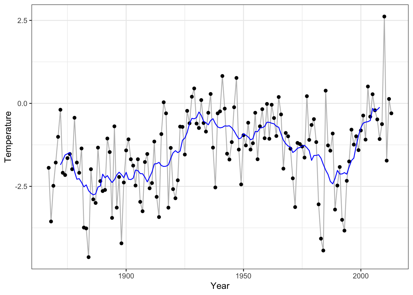
Figure 4.4: Annual average temperature in Nuuk smoothed using the running mean with \(k = 11\) neighbors. This time using a different implementation than in Figure 4.3.
The R function filter() (from the stats package) can be used to compute running
means and general moving averages using any weight vector. We compare our two
implementations to filter().
f_hat_filter <- stats::filter(nuuk$Temperature, rep(1/11, 11))
range(f_hat_filter - f_hat, na.rm = TRUE)
## [1] -4.441e-16 4.441e-16
range(f_hat_filter - run_mean(nuuk$Temperature, 11), na.rm = TRUE)## [1] -4.441e-16 1.332e-15Note that filter() uses the same boundary convention as used in run_mean().
A benchmark comparison between matrix-vector multiplication, run_mean() and filter()
gives the following table with median runtime in microseconds.
running_mean_bench <- bench::press(
  N = 2^(7:12),  # 128 to 4096
  {
    S <- run_mean_smoother(N, 11)
    y <- rnorm(N)
    bench::mark(
      matrix = c(S %*% y),
      run_mean = run_mean(y, k = 11),
      filter =  c(stats::filter(y, rep(1/11, 11)))
    )
  }
)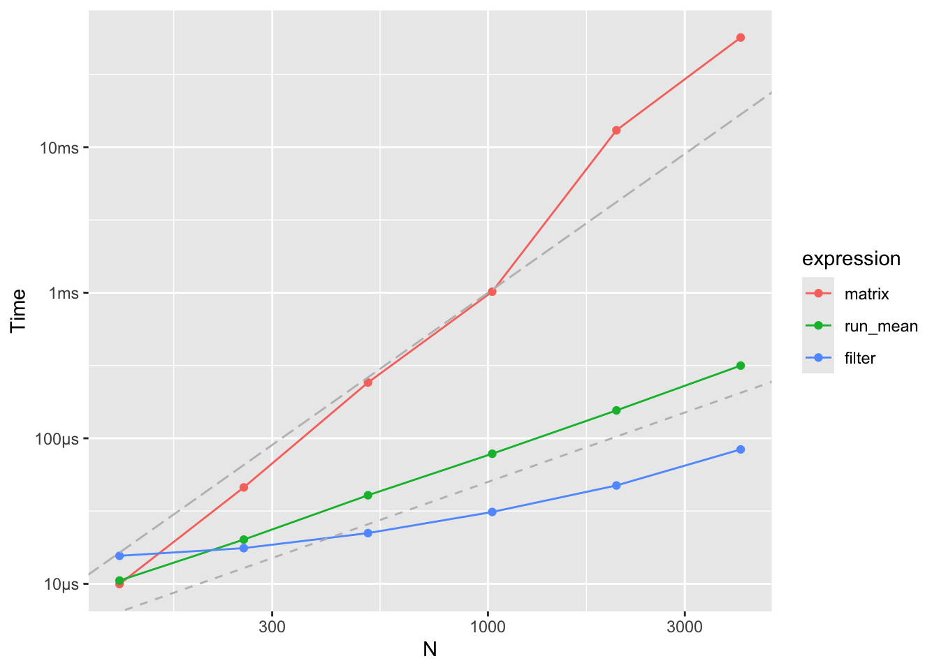
Figure 4.5: Running mean benchmarks
The matrix-vector computation is clearly much slower than the two alternatives,
and the time to construct the \(\mathbf{S}\)-matrix has not even been included
in the benchmark above. There is also a difference in how the matrix-vector
multiplication scales with the size of data compared to the alternatives.
Whenever the data size doubles the runtime approximately doubles for
both filter() and run_mean(), while it quadruples for the matrix-vector
multiplication. This shows the difference between an algorithm
that scales like \(O(N)\) and an algorithm that scales like \(O(N^2)\)
as the matrix-vector product does.
Despite that filter() is implementing a more general
algorithm than run_mean(), it is still faster, which reflects that
it is implemented in C and compiled.
4.1.3 Choose \(k\) by cross-validation
Cross-validation relies predictions of \(y_i\) from \(x_i\) for data points \((x_i, y_i)\) left out of the dataset when the predictor is fitted to data. Many (linear) smoothers have a natural definition of an “out-of-sample” prediction, that is, how \(\hat{f}(x)\) is computed for \(x\) not in the data. If so, it becomes possible to define
\[ \hat{f}^{-i}_i = \hat{f}^{-i}(x_i) \]
as the prediction at \(x_i\) using the smoother computed from data with \((x_i, y_i)\) excluded. However, here we directly define
\[ \hat{f}^{-i}_i = \sum_{j \neq i} \frac{S_{ij}y_j}{1 - S_{ii}} \]
for any linear smoother. This definition concurs with the “out-of-sample” predictor in \(x_i\) for most smoothers, but this has to be verified case-by-case.
The running mean is a little special in this respect. In the previous section, the running mean was only considered for odd \(k\) and using a symmetric neighbor definition. This is convenient when considering the running mean in the observations \(x_i\). When considering the running mean in any other point, a symmetric neighbor definition works better with an even \(k\). This is exactly what the definition of \(\hat{f}^{-i}_i\) above amounts to. If \(\mathbf{S}\) is the running mean smoother matrix for an odd \(k\), then \(\hat{f}^{-i}_i\) corresponds to symmetric \((k-1)\)-nearest neighbor smoothing excluding \((x_i, y_i)\) from the data.
Using the definition above, we get that the leave-one-out cross-validation squared error criterion becomes
\[ \mathrm{LOOCV} = \sum_{i=1}^N (y_i - \hat{f}^{-i}_i)^2 = \sum_{i=1}^N \left(\frac{y_i - \hat{f}_i}{1 - S_{ii}}\right)^2. \]
The important observation from the identity above is that LOOCV can be computed without actually computing all the \(\hat{f}^{-i}_i\).
For the running mean, all diagonal elements of the smoother matrix are identical.
We disregard boundary values (with the NA value), so to get
a comparable quantity across different choices of \(k\) we use mean() instead of
sum() in the implementation.
loocv <- function(k, y) {
  f_hat <- run_mean(y, k)
  mean(((y - f_hat) / (1 - 1/k))^2, na.rm = TRUE)
}
k <- seq(3, 40, 2)
CV <- sapply(k, loocv, y = nuuk$Temperature)
k_opt <- k[which.min(CV)]
ggplot(mapping = aes(k, CV)) + geom_line() +
  geom_vline(xintercept = k_opt, color = "red")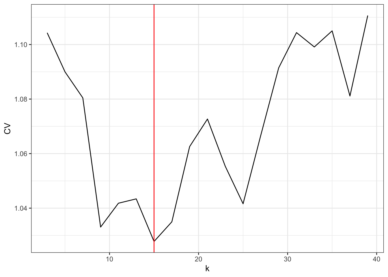
Figure 4.6: The leave-one-out cross-validation criterion for the running mean as a function of the number of neighbors \(k\).
The optimal choice of \(k\) is 15, but the LOOCV criterion jumps quite a lot up and down with changing neighbor size, and \(k = 9\) as well as \(k = 25\) give rather low values as well.
p_Nuuk +
#  geom_line(aes(y = run_mean(nuuk$Temperature, 9)), color = "red") +
geom_line(aes(y = run_mean(nuuk$Temperature, k_opt)), color = "blue") 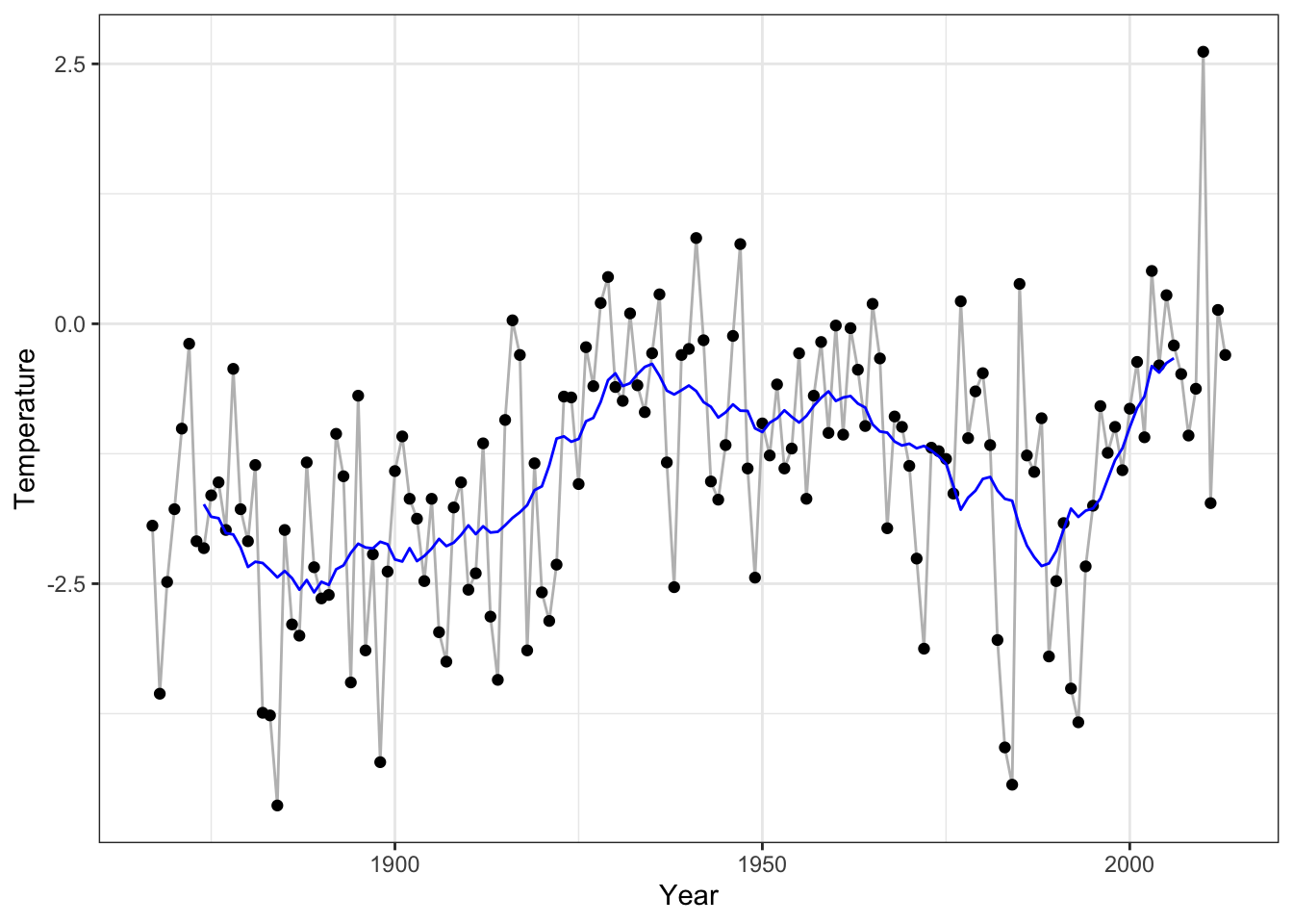
Figure 4.7: The \(k\)-nearest neighbor smoother with the optimal choice of \(k\) based on LOOCV (blue) and with \(k = 9\) (red) and \(k = 25\) (purple).
# geom_line(aes(y = run_mean(nuuk$Temperature, 25)), color = "purple")4.2 Fourier expansions
Introducing
\[ x_{k,m} = \frac{1}{\sqrt{n}} e^{2 \pi i k m / n}, \]
then
\[ \sum_{k=0}^{N-1} |x_{k,m}|^2 = 1 \]
and for \(m_1 \neq m_2\)
\[ \sum_{k=0}^{N-1} x_{k,m_1}\overline{x_{k,m_2}} = 0 \]
Thus \(\Phi = (x_{k,m})_{k,m}\) is an \(n \times n\) unitary matrix;
\[ \Phi^*\Phi = I \]
where \(\Phi^*\) is the conjugate transposed of \(\Phi\).
\(\hat{\beta} = \Phi^* y\) is the discrete Fourier transform of \(y\). It is the basis coefficients in the orthonormal basis given by \(\Phi\);
\[ y_k = \frac{1}{\sqrt{n}} \sum_{m=0}^{N-1} \hat{\beta}_m e^{2 \pi i k m / n} \]
or \(y = \Phi \hat{\beta}.\)
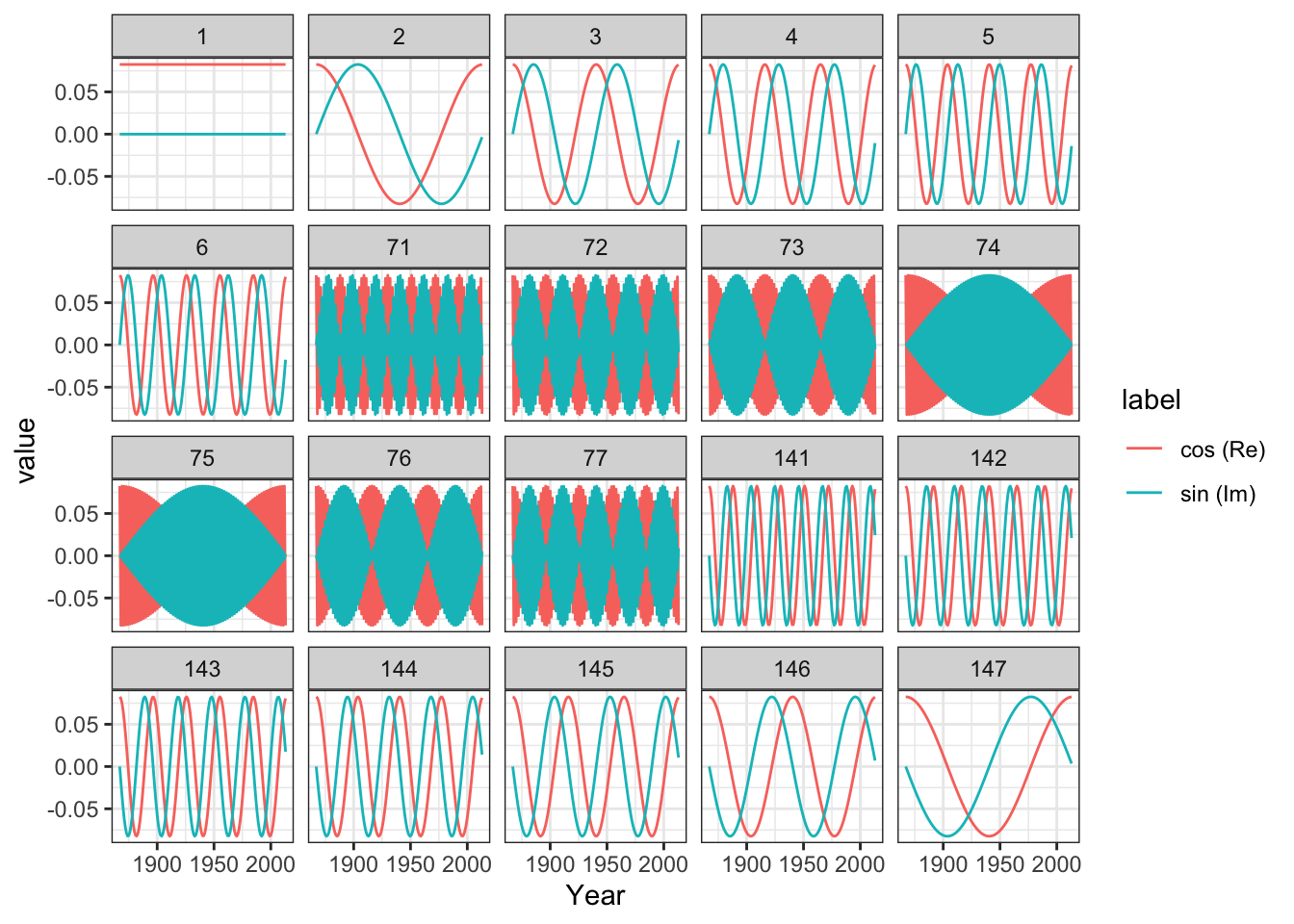
The matrix \(\Phi\) generates an interesting pattern.
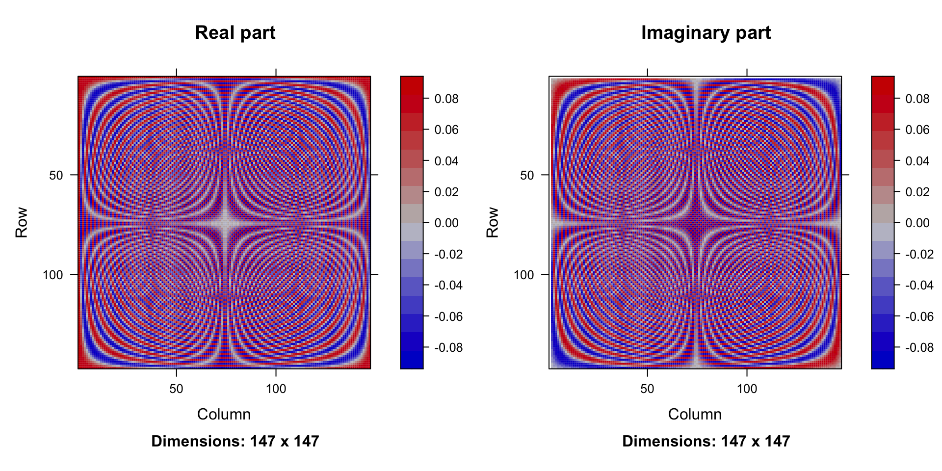
Columns in the matrix \(\Phi\):
We can estimate by matrix multiplication
betahat <- Conj(t(Phi)) %*% nuuk$Temperature # t(Phi) = Phi for Fourier bases
betahat[c(1, 2:4, 73, N:(N - 2))]
## [1] -17.24696+0.0000i -2.46429+2.3871i 3.54813+0.9099i 1.67214+0.7414i
## [5] 0.03212+0.7090i -2.46429-2.3871i 3.54813-0.9099i 1.67214-0.7414iFor real \(y\) it holds that \(\hat{\beta}_0\) is real, and the symmetry
\[ \hat{\beta}_{N-m} = \hat{\beta}_m^* \]
holds for \(m = 1, \ldots, N - 1\). (For \(N\) even, \(\hat{\beta}_{N/2}\) is real too).
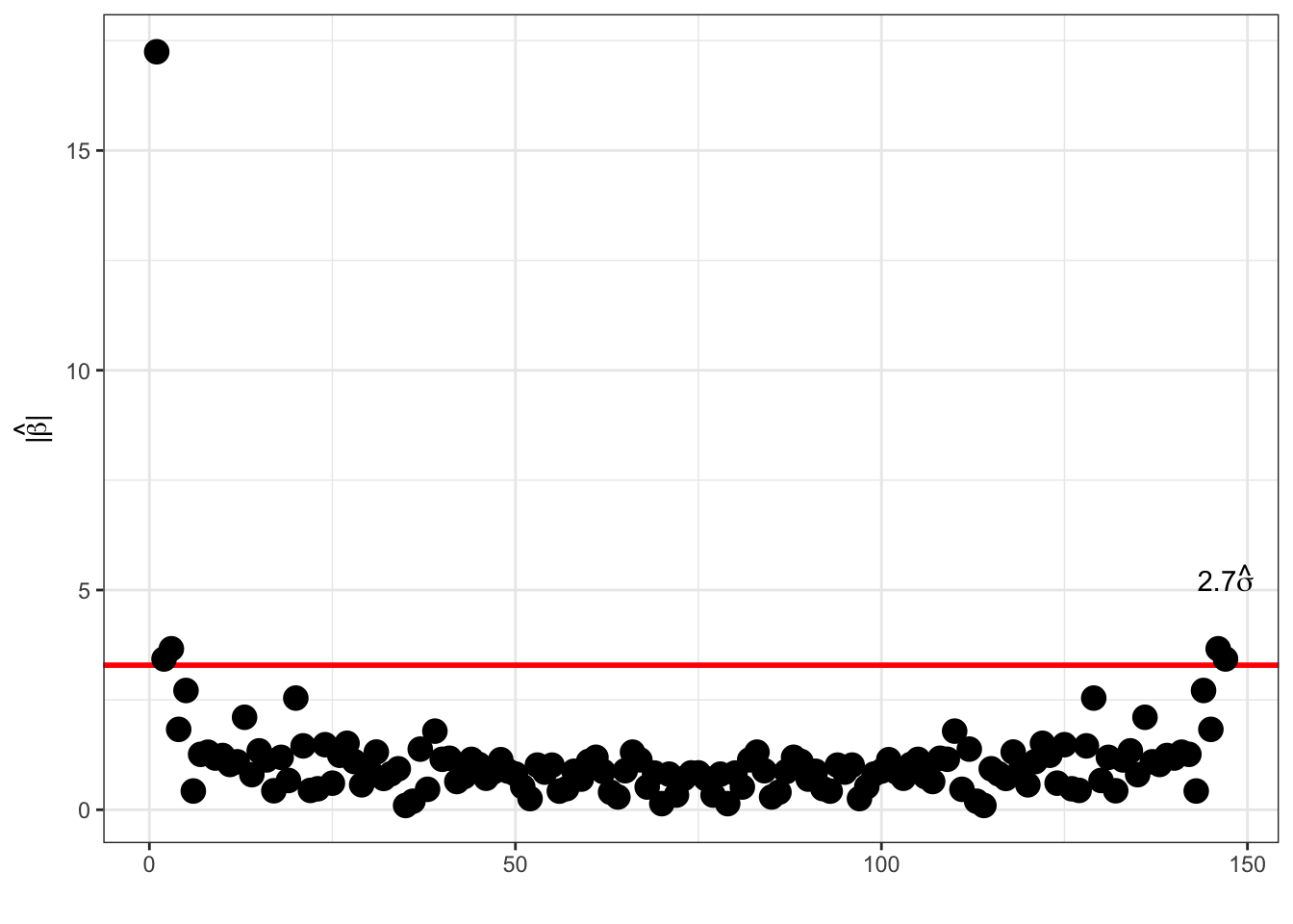
Modulus distribution:
Note that for \(m \neq 0, N/2\), \(\beta_m = 0\) and \(y \sim \mathcal{N}(\Phi\beta, \sigma^2 I_N)\) then
\[(\mathrm{Re}(\hat{\beta}_m), \mathrm{Im}(\hat{\beta}_m))^T \sim \mathcal{N}\left(0, \frac{\sigma^2}{2} I_2\right),\]
hence \[|\hat{\beta}_m|^2 = \mathrm{Re}(\hat{\beta}_m)^2 + \mathrm{Im}(\hat{\beta}_m)^2 \sim \frac{\sigma^2}{2} \chi^2_2,\] that is, \(P(|\hat{\beta}_m| \geq 1.73 \sigma) = 0.05.\) There is a clear case of multiple testing if we use this threshold at face value, and we would expect around \(0.05 \times n/2\) false positive if there is no signal at all. Lowering the probability using the Bonferroni correction yields a threshold of around \(2.7 \sigma\) instead.
Thresholding Fourier:
The coefficients are not independent (remember the symmetry), and one can alternatively consider \[\hat{\gamma}_m = \sqrt{2} \mathrm{Re}(\hat{\beta}_m) \quad \text{and} \quad \hat{\gamma}_{n' + m} = - \sqrt{2} \mathrm{Im}(\hat{\beta}_m)\] for \(1 \leq m < n / 2\). Here \(n' = \lfloor n / 2 \rfloor\). Here, \(\hat{\gamma}_0 = \hat{\beta}_0\), and \(\hat{\gamma}_{n/2} = \hat{\beta}_{n/2}\) for \(n\) even.
These coefficients are the coefficients in a real cosine, \(\sqrt{2} \cos(2\pi k m / n)\), and sine, \(\sqrt{2} \sin(2\pi k m / n)\), basis expansion, and they are i.i.d. \(\mathcal{N}(0, \sigma^2)\) distributed.
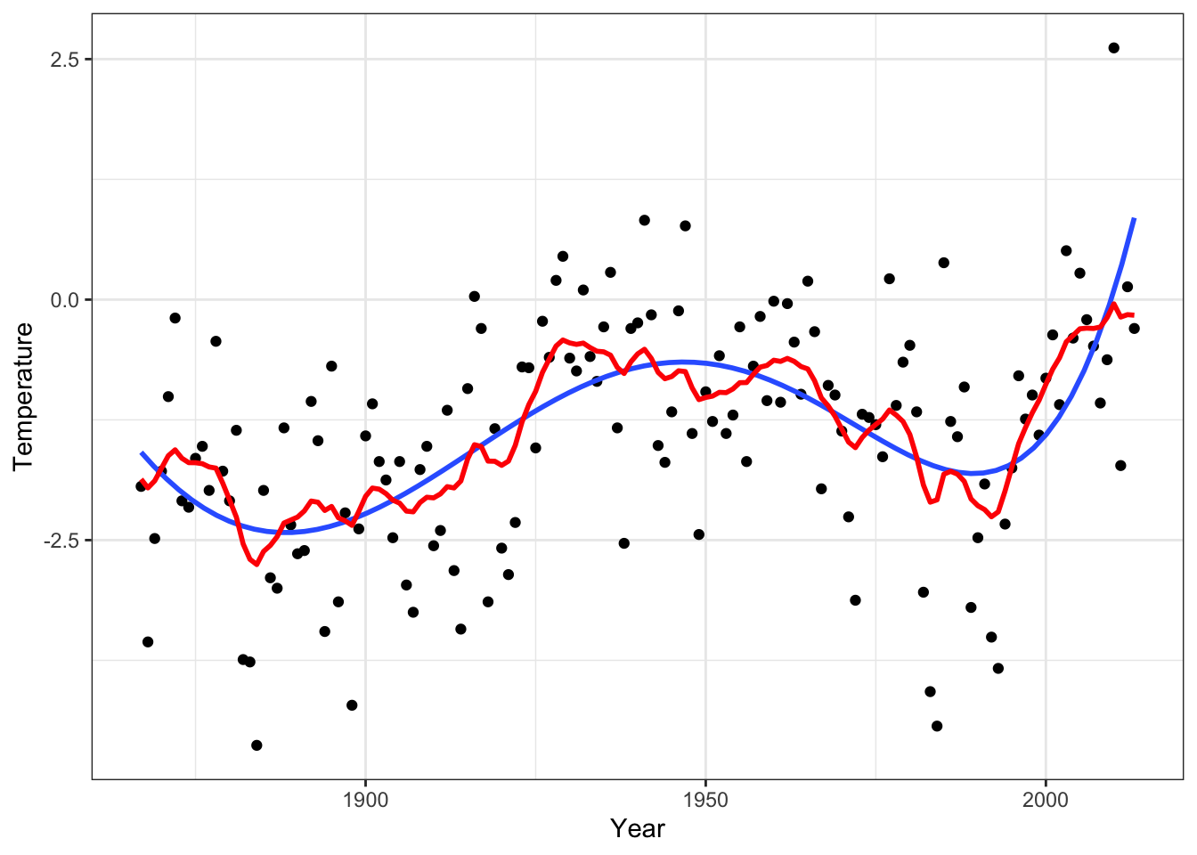
Thresholding Fourier:
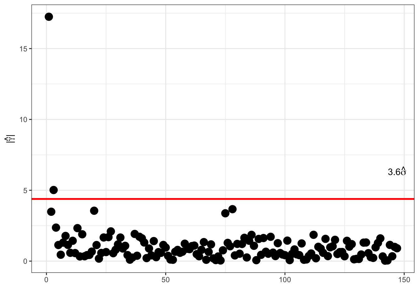
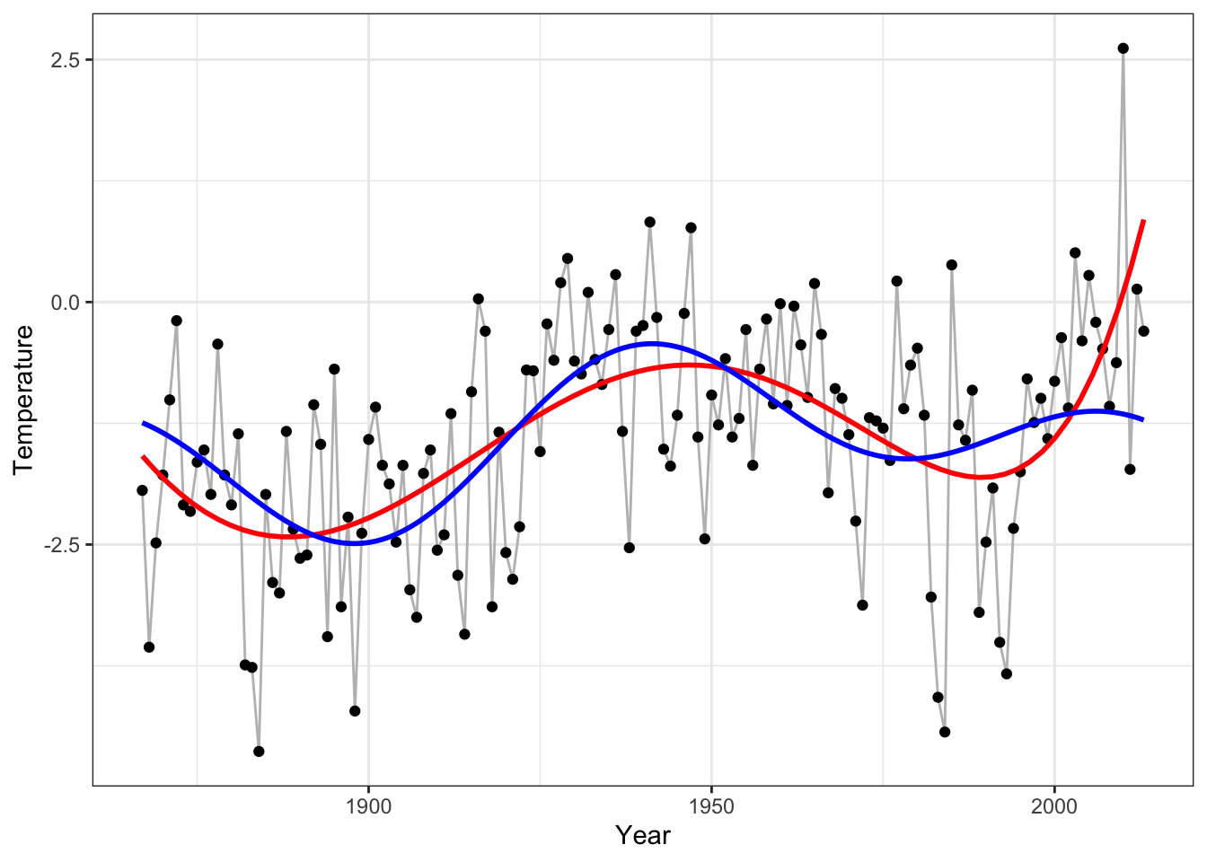
Figure 4.8: Fourier based smoother by thresholding (blue) and polynomial fit of degree 5 (red).
What is the point using the discrete Fourier transform? The point is that the discrete Fourier transform can be computed via the fast Fourier transform (FFT), which has an \(O(n\log(n))\) time complexity. The FFT works optimally for \(n = 2^p\).
## [1] -17.247+0.0000i -2.464+2.3871i 3.548+0.9099i 1.672+0.7414i
betahat[1:4]## [1] -17.247+0.0000i -2.464+2.3871i 3.548+0.9099i 1.672+0.7414i4.3 Kalman smoothing and filtering
gauss_process_kernel <- function(N, alpha, eta) {
  K <- function(x) alpha^(abs(x)) / (1 - alpha^2)
  eta * outer(1:N, 1:N, function(i, j) K(i - j))
}

gauss_process_smoother <- function(y, Sigma_x, sigmasq, ...) {
  N <- length(y)
  if (missing(Sigma_x)) {
    Sigma_x <- gauss_process_kernel(N, ...)
  }
  Sigma_x %*% solve(Sigma_x + diag(rep(sigmasq, N)), y)
}
eta <- 1
alpha <- 0.9
sigmasq <- 20
y <- nuuk$Temperature
mx <- mean(y)
f_smooth <- gauss_process_smoother(y - mx, sigmasq = sigmasq, alpha = alpha, eta = eta) + mx
p_Nuuk +
  geom_line(aes(y = f_smooth), lwd = 1, color = "red")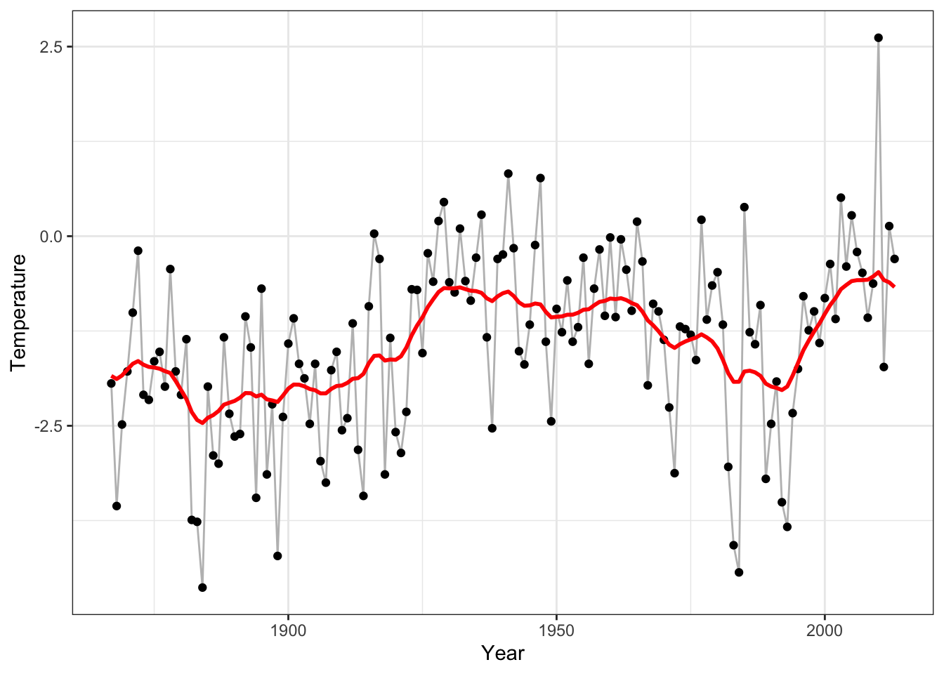
gauss_process_loglik <- function(par, y) {
  sigmasq <- par[1]
  alpha <- par[2]
  eta <- par[3]
  N <- length(y)
  Sigma <- gauss_process_kernel(N, alpha, eta) + diag(rep(sigmasq, N))
  d <- svd(Sigma, 0, 0)$d
  drop(y %*% solve(Sigma, y) + sum(log(d)))
}
gauss_process_loglik(c(1, 0.5, 1), y)## [1] 252.4
optim(c(1, 0.5, 1), gauss_process_loglik, method = "L-BFGS-B", lower = c(0.01, 0.01, 0.01), upper = c(Inf, 0.99, Inf), y = y - mx)## $par
## [1] 0.7921 0.8879 0.1427
##
## $value
## [1] 163.6
##
## $counts
## function gradient
## 20 20
##
## $convergence
## [1] 0
##
## $message
## [1] "CONVERGENCE: REL_REDUCTION_OF_F <= FACTR*EPSMCH"
gauss_process_loocv <- function(par, y) {
  sigmasq <- par[1]
  alpha <- par[2]
  eta <- par[3]
  N <- length(y)
  Sigma_x <- gauss_process_kernel(N, alpha, eta)
  S <- Sigma_x %*% solve(Sigma_x  + diag(rep(sigmasq, N)))
  f_hat <- S %*% y
  sum(((y - f_hat) / (1- diag(S)))^2)
}
gauss_process_loocv(c(1, 0.5, 1), y)## [1] 196.4
optim(c(1, 0.5, 1), gauss_process_loocv, method = "L-BFGS-B", lower = c(0.01, 0.01, 0.01), upper = c(Inf, 0.99, Inf), y = y - mx)## $par
## [1] 1.0335 0.6688 1.0072
##
## $value
## [1] 145.1
##
## $counts
## function gradient
## 13 13
##
## $convergence
## [1] 0
##
## $message
## [1] "CONVERGENCE: REL_REDUCTION_OF_F <= FACTR*EPSMCH"
sigmasq <- 0.8
alpha <- 0.89
eta <- 0.14

# sigmasq <- 0.88
# alpha <- 0.98
# eta <- 0.06

y <- nuuk$Temperature
# mx <- mean(y)
mx <- 0
f_smooth <- gauss_process_smoother(y - mx, sigmasq = sigmasq, alpha = alpha, eta = eta) + mx
p_Nuuk +
  geom_line(aes(y = f_smooth), lwd = 1, color = "red") +
  geom_line(aes(y = run_mean(nuuk$Temperature, k_opt)), color = "blue", lwd = 1)
## Warning: Use of `nuuk$Temperature` is discouraged.
## ℹ Use `Temperature` instead.## Warning: Removed 14 rows containing missing values or values outside the scale
## range (`geom_line()`).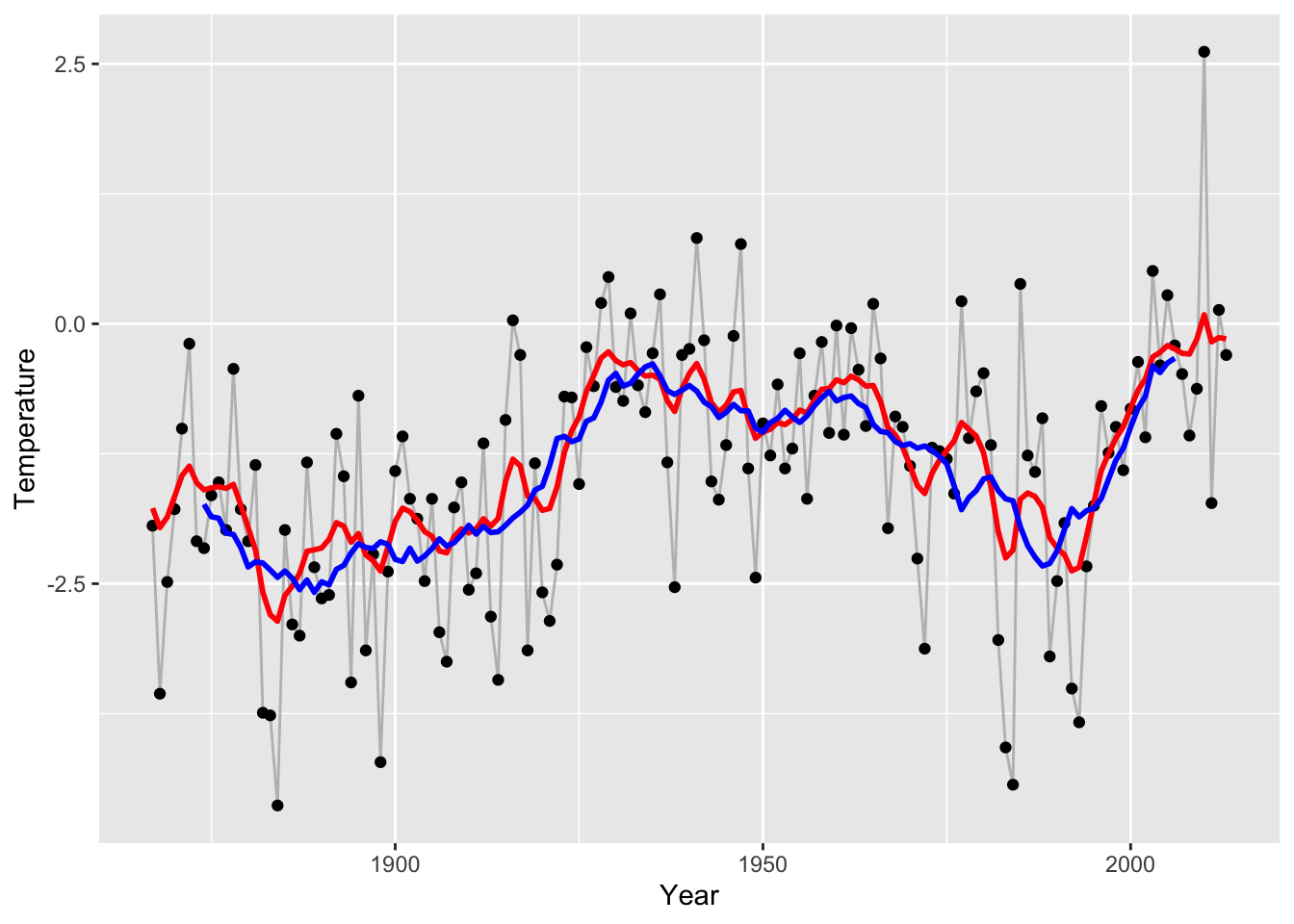
4.3.1 AR(1) Kalman smoothing
The simplest example with an efficient Kalman smoother is the AR(1)-model, where we assume an equidistant time grid (that is, \(x_i = i\)). Suppose that \(|\alpha| < 1\), \(f_1 = U_1 / \sqrt{1 - \alpha^2}\) and
\[ f_i = \alpha f_{i-1} + \tau U_i \]
for \(i = 2, \ldots, n\) with \(U = (U_1, \ldots, U_N) \sim \mathcal{N}(0, I)\).
We have \(\cov(f_i, f_j) = \tau^2 \alpha^{|i-j|} / (1 - \alpha^2)\), thus we can find \(\mathbf{K}\), and by (3.2) we have
\[ \E(\mathbf{f} \mid \mathbf{Y} = \mathbf{y}) = (I + \sigma^2 \mathbf{K}^{-1})^{-1} \mathbf{y} \]
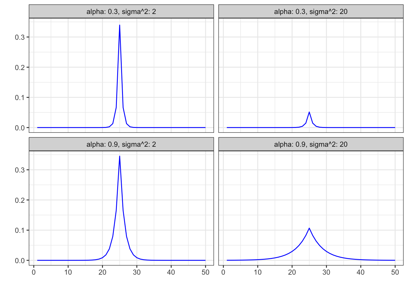
Figure 4.9: Gaussian smoother matrix \(S_{25,j}\) with \(\alpha = 0.3, 0.9\), \(\sigma^2 = 2, 20\)
From the identity \(U_i = f_i - \alpha f_{i-1}\) it follows that \(U = A \mathbf{f}\) where
\[ A = \left( \begin{array}{cccccc} \sqrt{1 - \alpha^2} & 0 & 0 & \ldots & 0 & 0 \\ -\alpha & 1 & 0 & \ldots & 0 & 0 \\ 0 & -\alpha & 1 & \ldots & 0 & 0 \\ \vdots & \vdots & \vdots & \ddots & \vdots & \vdots \\ 0 & 0 & 0 & \ldots & 1 & 0 \\ 0 & 0 & 0 & \ldots & -\alpha & 1 \\ \end{array}\right), \]
This gives \(\tau^2 I = V(U) = A \mathbf{K} A^T\), hence
\[ \mathbf{K}^{-1} = \frac{1}{\tau^2} (A^{-1}(A^T)^{-1})^{-1} = \frac{1}{\tau^2} A^T A. \]
We have shown that
\[ \mathbf{K}^{-1} = \frac{1}{\tau^2} \left( \begin{array}{cccccc} 1 & -\alpha & 0 & \ldots & 0 & 0 \\ -\alpha & 1 + \alpha^2 & -\alpha & \ldots & 0 & 0 \\ 0 & -\alpha & 1 + \alpha^2 & \ldots & 0 & 0 \\ \vdots & \vdots & \vdots & \ddots & \vdots & \vdots \\ 0 & 0 & 0 & \ldots & 1 + \alpha^2 & -\alpha \\ 0 & 0 & 0 & \ldots & -\alpha & 1 \\ \end{array}\right). \]
Hence letting \(\eta = \sigma^2 / \tau^2\) and \(\gamma_0 = 1 + \eta\), \(\gamma = 1 + \eta (1 + \alpha^2)\) and \(\rho = - \eta \alpha\),
\[ I + \sigma^2 \mathbf{K}^{-1} = \left( \begin{array}{cccccc} \gamma_0 & \rho & 0 & \ldots & 0 & 0 \\ \rho & \gamma & \rho & \ldots & 0 & 0 \\ 0 & \rho & \gamma & \ldots & 0 & 0 \\ \vdots & \vdots & \vdots & \ddots & \vdots & \vdots \\ 0 & 0 & 0 & \ldots & \gamma & \rho \\ 0 & 0 & 0 & \ldots & \rho & \gamma_0 \\ \end{array}\right) \]
is a tridiagonal matrix.
The equation
\[ \left( \begin{array}{cccccc} \gamma_0 & \rho & 0 & \ldots & 0 & 0 \\ \rho & \gamma & \rho & \ldots & 0 & 0 \\ 0 & \rho & \gamma & \ldots & 0 & 0 \\ \vdots & \vdots & \vdots & \ddots & \vdots & \vdots \\ 0 & 0 & 0 & \ldots & \gamma & \rho \\ 0 & 0 & 0 & \ldots & \rho & \gamma_0 \\ \end{array}\right) \left( \begin{array}{c} f_1 \\ f_2 \\ f_3 \\ \vdots \\ f_{N-1} \\ f_N \end{array}\right) = \left(\begin{array}{c} y_1 \\ y_2 \\ y_3 \\ \vdots \\ y_{N-1} \\ y_N \end{array}\right) \]
can be solved by a forward and backward sweep.
Forward sweep:
- Set \(\rho_1' = \rho / \gamma_0\) and \(y_1' = y_1 / \gamma_0\),
- then recursively \[\rho_i' = \frac{\rho}{\gamma - \rho \rho_{i-1}'} \quad \text{and} \quad y_i' = \frac{y_i - \rho y_{i-1}'}{\gamma - \rho \rho_{i-1}'}\] for \(i = 2, \ldots, N-1\)
- and finally \[y_N' = \frac{y_N - \rho y_{N-1}'}{\gamma_0 - \rho \rho_{N-1}'}.\]
By the forward sweep the equation is transformed to
\[ \left( \begin{array}{cccccc} 1 & \rho_1' & 0 & \ldots & 0 & 0 \\ 0 & 1 & \rho_2' & \ldots & 0 & 0 \\ 0 & 0 & 1 & \ldots & 0 & 0 \\ \vdots & \vdots & \vdots & \ddots & \vdots & \vdots \\ 0 & 0 & 0 & \ldots & 1 & \rho_{N-1}' \\ 0 & 0 & 0 & \ldots & 0 & 1 \\ \end{array}\right) \left( \begin{array}{c} f_1 \\ f_2 \\ f_3 \\ \vdots \\ f_{N-1} \\ f_N \end{array}\right) = \left(\begin{array}{c} y_1' \\ y_2' \\ y_3' \\ \vdots \\ y_{N-1}' \\ y_N' \end{array}\right), \]
which is then solved by backsubstitution from below; \(f_N = y_N'\) and
\[ f_{i} = y_i' - \rho_{i}' f_{i+1}, \quad i = N-1, \ldots, 1. \]
4.3.2 Implementation
#include <Rcpp.h>
using namespace Rcpp;
// [[Rcpp::export]]
NumericVector kalman_smooth(NumericVector y, double alpha, double eta) {
  double tmp, gamma0 = 1 + eta, rho = - eta * alpha;
  double gamma = 1 + eta * (1 + alpha * alpha);
  int N = y.size();
  NumericVector f(N), rhop(N - 1);
  rhop[0] = rho / gamma0;
  f[0] = y[0] / gamma0;
  for(int i = 1; i < N - 1; ++i) { /* Forward sweep */
    tmp = (gamma - rho * rhop[i - 1]);
    rhop[i] = rho / tmp;
    f[i] = (y[i] - rho * f[i - 1]) / tmp;
  }
  f[N - 1] = (y[N - 1] - rho * f[N - 2]) / (gamma0 - rho * rhop[N - 2]);
  for(int i = N - 2; i >= 0; --i) { /* Backsubstitution */
    f[i] = f[i] - rhop[i] * f[i + 1];
  }
  return f;
}
Result, \(\alpha = 0.95\), \(\sigma^2 = 50\)
Comparing results
Sigma <- outer(1:N, 1:N,
               function(i, j) alpha^(abs(i - j))) / (1 - alpha^2)
Smooth <- Sigma %*% solve(Sigma + eta * diag(N))


xi <- mean(nuuk$Temperature)
f_smooth <- Smooth %*% (nuuk$Temperature - xi) + xi
p_Nuuk +
  geom_line(aes(y = f_smooth), lwd = 1, color = "red")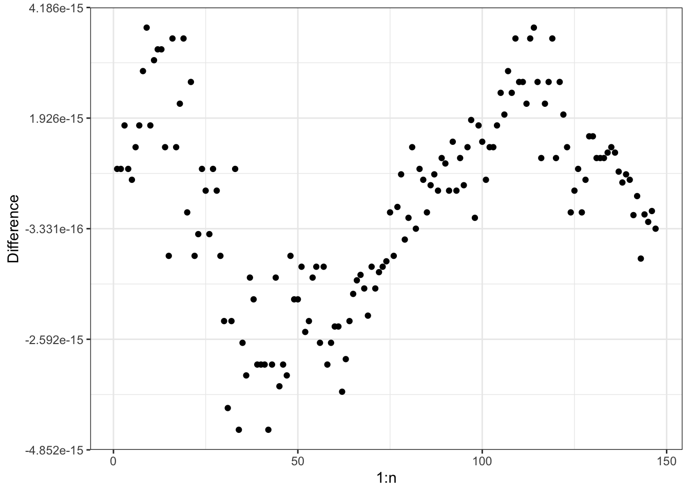
ggplot(mapping = aes(1:N, Smooth %*% (nuuk$Temperature - xi) - f_smooth + xi)) +
  geom_point() +
  ylab("Difference")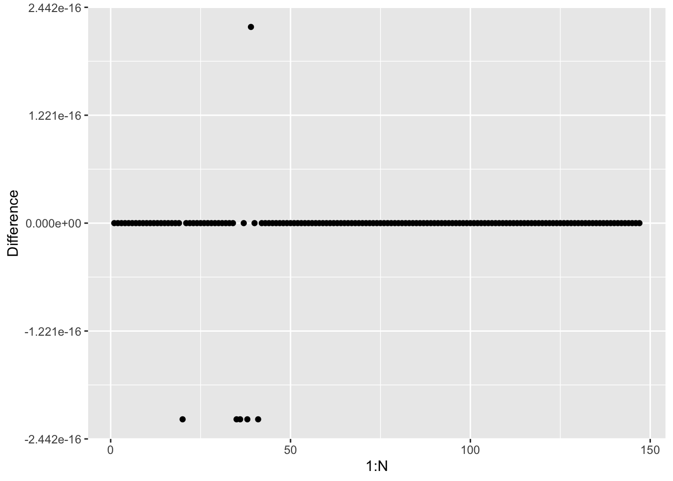
Note that the forward sweep computes \(\hat{f}_N = E(f_N \mid \mathbf{Y} = \mathbf{y})\), and from this, the backsubstitution solves the smoothing problem of computing \(E(\mathbf{f} \mid \mathbf{Y} = \mathbf{y})\).
The Gaussian process used here (the AR(1)-process) is not very smooth and nor is the smoothing of the data. This is related to the kernel function \(K(s) = \alpha^{|s|}\) being non-differentiable in 0.
Many smoothers are equivalent to a Gaussian process smoother with an appropriate choice of kernel. Not all have a simple inverse covariance matrix and a Kalman filter algorithm.
4.3.3 The Kalman filter
#include <Rcpp.h>
using namespace Rcpp;
// [[Rcpp::export]]
NumericVector kalman_filter(NumericVector y, double alpha, double eta) {
  double tmp, gamma0 = 1 + eta, rho = - eta * alpha, yp;
  double gamma = 1 + eta * (1 + alpha * alpha);
  int N = y.size();
  NumericVector f(N), rhop(N);
  rhop[0] = rho / gamma0;
  yp = y[0] / gamma0;
  f[0] = y[0] / (1 + eta * (1 - alpha * alpha));
  for(int i = 1; i < N; ++i) {
    tmp = (gamma - rho * rhop[i - 1]);
    rhop[i] = rho / tmp;
    /* Note differences when compared to smoother */
    f[i] = (y[i] - rho * yp) / (gamma0 - rho * rhop[i - 1]);
    yp = (y[i] - rho * yp) / tmp;
  }
  return f;
}
Result, \(\alpha = 0.95\), \(\sigma^2 = 10\)