5 Random number generation
This chapter deals with algorithms for generating random numbers from a probability distribution on \(\mathbb{R}\) or a subset thereof. Two applications of random number generation within statistics are: simulation studies and Monte Carlo integration. A simulation study investigates distributional properties of statistical procedures, and such studies have become an indispensable experimental part of the development of statistical methodology. Monte Carlo integration is a more specific application of random number generation as a way to numerically compute a probability or an integral.
Random number generators are also used when implementing randomization protocols in randomized controlled trials, for resampling and subsampling based statistical methods, such as bootstrapping, and in other randomized algorithms, such as stochastic optimization algorithms. There are likewise important applications of random number generators outside of statistics, e.g., within cryptography. We will not pursue all these different applications, nor will we deal with the design and implementation of general simulation studies.
In this chapter the focus is on the generation of a single random number or an i.i.d. sequence of random numbers. In particular, how pseudorandom number generators are implemented and used to approximate sampling of i.i.d. random variables that are uniformly distributed on \((0, 1)\). Section 5.2 illustrates how simulation from other distributions than the uniform can be obtained from pseudorandom number generators via transformations.
Chapter 6 treats rejection sampling, in particular for distributions on \(\mathbb{R}\). Chapter 7 deals with Monte Carlo integration in greater detail, in particular how to assess the precision of computations based on random number generation. Chapters 11 and 12 rely on (pseudo)random numbers as an integral part of any stochastic optimization algorithm.
5.1 Pseudorandom number generators
Most simulation algorithms are based on algorithms for generating pseudorandom uniformly distributed variables in \((0, 1)\). Such pseudorandom variables all arise from deterministic sequences of numbers initiated by a seed. A classical example of a pseudorandom integer generator is the linear congruential generator. A sequence of numbers from this generator is computed iteratively by
\[ x_{n+1} = (a x_n + c) \text{ mod m} \]
for integer parameters \(a\), \(c\) and \(m\). The seed \(x_1\) is a number between \(0\) and \(m - 1\), and the resulting sequence is in the set \(\{0, \ldots, m - 1\}\). The ANSI C standard specifies the choices \(m = 2^{31}\), \(a = 1,103,515,245\) and \(c = 12,345\). The generator is simple to understand and implement but has been superseded by much better generators.
Pseudorandom number generators are generally defined in terms of a finite state space \(\mathcal{Z}\) and a one-to-one map \(f : \mathcal{Z} \to \mathcal{Z}\). The generator produces a sequence in \(\mathcal{Z}\) iteratively from the seed \(\mathbf{z}_1 \in \mathcal{Z}\) by
\[ \mathbf{z}_n = f(\mathbf{z}_{n-1}). \]
Pseudorandom integers are typically obtained as
\[ x_n = h(\mathbf{z}_n) \]
for a map \(h : \mathcal{Z} \mapsto \mathbb{Z}\). If the image of \(h\) is in the set \(\{0, 1, \ldots, 2^{w} - 1\}\) of \(w\)-bit integers, pseudorandom numbers in \([0, 1)\) are typically obtained as
\[ x_n = 2^{-w} h(\mathbf{z}_n). \]
In R, the default pseudorandom number generator is the 32-bit Mersenne Twister, which generates integers in the range
\[ \{0, 1, \ldots, 2^{32} -1\}. \]
The state space is
\[ \mathcal{Z} = \{0, 1, \ldots, 2^{32} -1\}^{624}, \]
that is, a state is a 624 dimensional vector of 32-bit integers. The function \(f\) is of the form
\[ f(\mathbf{z}) = (z_2, z_3, \ldots, z_{623}, f_{624}(z_1, z_2, z_{m + 1})), \]
for \(1 \leq m < 624\), and \(h\) is a function of \(z_{624}\) only. The standard choice \(m = 397\) is used in the R implementation. The function \(f_{624}\) is a bit complicated. It includes what is known as the twist transformation, and it requires additional parameters. The period of the generator is the astronomical number
\[ 2^{32 \times 624 - 31} - 1 = 2^{19937} - 1, \]
which is a Mersenne prime. Moreover, all combinations of consecutive integers up to dimension 623 occur equally often in a period, and empirical tests of the generator demonstrate that it has good statistical properties, though it is known to fail some tests.
In R you can set the seed using the function set.seed() that takes an
integer argument and produces an element in the state space. The argument
given to set.seed() is not the actual seed, and set.seed() computes a
valid seed for any pseudorandom number generator that R is using,
whether it is the Mersenne Twister or not. Thus the use of set.seed() is
the safe and recommended way of setting a seed.
The actual seed (together with some additional information) can be accessed
via the vector .Random.seed. Its first entry, .Random.seed[1], encodes the
pseudorandom number generator used as well as the generator for
Gaussian variables and discrete uniform variables. This
information is decoded by RNGkind().
RNGkind()## [1] "Mersenne-Twister" "Inversion" "Rejection"For the Mersenne Twister,
.Random.seed[3:626] contains the vector in the state space, while
.Random.seed[2] contains the “current position” in the state vector.
The implementation needs a position variable because it does 624 updates of the
state vector at a time and then runs through those values sequentially
before the next update. This is equivalent to but more efficient than
implementing the position shifts explicitly as in the definition of \(f\) above.
set.seed(27112015)           # Computes a new seed from an integer
oldseed <- .Random.seed[-1]  # The actual seed
.Random.seed[1]              # Encoding of generators used (stays fixed)
## [1] 10403
.Random.seed[2] # Start position after new seed is 624## [1] 624
tmp <- runif(1)
tmp
## [1] 0.7793Every time a random number is generated, by runif() as above or by any other
R function relying on the default pseudorandom number generator, the same underlying
sequence of pseudorandom numbers is used, and the state vector stored in
.Random.seed is updated accordingly.
head(oldseed, 5)## [1] 624 -1660633125 -1167670944 1031453153 815285806
head(.Random.seed[-1], 5) # State vector and position updated## [1] 1 -696993996 -1035426662 -378189083 -745352065## [1] 0.7793 0.5613
head(.Random.seed[-1], 5) # State vector unchanged, position updated## [1] 2 -696993996 -1035426662 -378189083 -745352065Resetting the seed will restart the pseudorandom number generator with the same seed and result in the same sequence of random numbers.
## [1] 624 -1660633125 -1167670944 1031453153 815285806
head(oldseed, 5) # Same as current .Random.seed## [1] 624 -1660633125 -1167670944 1031453153 815285806
runif(1) # Same as tmp## [1] 0.7793Note that when using any of the standard R generators, any value of \(0\) or \(1\) returned by the underlying pseudorandom uniform generator is adjusted to be in \((0,1)\). Uniform random variables are thus guaranteed to be in \((0, 1)\).
Some of the random number generators implemented in R use more than one pseudorandom number per variable. This is, for instance, the case when we simulate gamma distributed random variables.
## [1] 1.193
head(.Random.seed[-1], 5) # Position changed to 2## [1] 2 -696993996 -1035426662 -378189083 -745352065
rgamma(1, 1) # A single gamma distributed random number## [1] 0.2795
head(.Random.seed[-1], 5) # Position changed to 5## [1] 5 -696993996 -1035426662 -378189083 -745352065In the example above, the first gamma variable required two pseudorandom numbers, while the second required three pseudorandom numbers. The detailed explanation is given in Section 6, where it is shown how to generate random variables from the gamma distribution via rejection sampling. This requires as a minimum two pseudorandom numbers for every gamma variable generated.
The development of high quality pseudorandom number generators is a research field in itself. This is particularly true if one needs theoretical guarantees for randomized algorithms or cryptographically secure generators. For scientific computations and simulations, reproducibility and speed are more important than cryptographic security—if the generator has acceptable statistical properties. It is, nevertheless, not easy to invent a good generator, and the field is still developing. For a generator to be seriously considered, its mathematical properties should be well understood, and it should pass (most) tests in standardized test suites such as TestU01, see L’Ecuyer and Simard (2007).
R provides a couple of alternatives to the Mersenne Twister,
see ?RNG, but there is no compelling reason to switch to any of those for ordinary
use. They are mostly available for historical reasons.
One exception is the L’Ecuyer-CMRG generator, which is useful when
independent pseudorandom sequences are needed for parallel computations.
Though the Mersenne Twister is a widely used pseudorandom number generator, it has some known shortcomings (O’Neill 2018), see also (O’Neill 2014). In the following two sections we discuss alternatives to the standard pseudorandom number generators available in R.
5.1.1 Implementing a pseudorandom number generator
This section dives into low-level aspects of an efficient implementation of a pseudorandom number generator via Rcpp. This involves turning the generator into the default generator used by R. The implementation illustrates bit-level C/C++ programming techniques, some aspects of R’s interface to compiled code, and how users can make compiled code available. However, the section can safely be skipped in a first reading, and other parts of the book do not rely explicitly on material in this section.
The family of shift-register generators and their variations are considered to be high quality alternatives to the Mersenne Twister, and to be both simpler and faster. At the time of writing such generators are, however, not available from the base R package.
Shift-register generators are based on linear transformations of the bit representation of integers. Three particular transformations are typically composed; the \(\mathrm{Lshift}\) and \(\mathrm{Rshift}\) operators and the bitwise \(\mathrm{xor}\) operator. Let \(z = [z_{31}, z_{30}, \ldots, z_0]\) with \(z_i \in \{0, 1\}\) denote the bit representation of a 32-bit (unsigned) integer \(z\) (ordered from most significant bit to least significant bit). That is,
\[ z = z_{31} 2^{31} + z_{30} 2^{30} + \ldots + z_2 2^2 + z_1 2^{1} + z_0. \]
Then the left shift operator is defined as
\[ \mathrm{Lshift}(z) = [z_{30}, z_{29}, \ldots, z_0, 0], \]
and the right shift operator is defined as
\[ \mathrm{Rshift}(z) = [0, z_{31}, z_{30}, \ldots, z_1]. \]
The bitwise xor operator is defined as
\[ \mathrm{xor}(z, z') = [\mathrm{xor}(z_{31},z_{31}') , \mathrm{xor}(z_{30}, z_{30}'), \ldots, \mathrm{xor}(z_0, z_0')] \]
where \(\mathrm{xor}(0, 0) = \mathrm{xor}(1, 1) = 0\) and \(\mathrm{xor}(1, 0) = \mathrm{xor}(0, 1) = 1\). Thus a transformation could be of the form
\[ \mathrm{xor}(z, \mathrm{Rshift}^2(z)) = [\mathrm{xor}(z_{31}, 0) , \mathrm{xor}(z_{30}, 0), \mathrm{xor}(z_{29}, z_{31}), \ldots, \mathrm{xor}(z_0, z_2)]. \]
One example of a shift-register based generator is Marsaglia’s xorwow algorithm, Marsaglia (2003). In addition to the shift and xor operations, the output of this generator is perturbed by a sequence of integers with period \(2^{32}\). The state space of the generator is
\[ \{0, 1, \ldots, 2^{32} -1\}^{5} \]
with
\[ f(\mathbf{z}) = (z_1 + 362437 \ (\mathrm{mod}\ 2^{32}), f_1(z_5, z_2), z_2, z_3, z_4), \]
and
\[ h(\mathbf{z}) = 2^{-32} (z_1 + z_2). \]
The number 362437 is Marsaglia’s choice for generating what he calls a Weyl sequence, but any odd number will do. The function \(f_1\) is given as
\[\begin{align*} \overline{z} & = \mathrm{xor}(z, \mathrm{Rshift}^2(z)) \\ f_1(z, z') & = \mathrm{xor}(\overline{z}, \mathrm{xor}(z', \mathrm{xor}(\mathrm{Lshift}^4(z'), \mathrm{Lshift}(\overline{z})))). \end{align*}\]
This may look intimidating, but all the operations are very elementary. Take the numbers \(z = 123456\) and \(z' = 87654321\), say. Then we can find their binary representations in R, in the bit order as above, as follows:
z <- intToBits(123456) |> as.integer() |> rev()
zp <- intToBits(87654321) |> as.integer() |> rev()
cat("z  = ", z, "\n", "z' = ", zp, sep = "")
## z = 00000000000000011110001001000000
## z' = 00000101001110010111111110110001The intermediate value \(\overline{z} = \mathrm{xor}(z, \mathrm{Rshift}^2(z))\) is computed as follows:
\[ \begin{array}{ll} z & \texttt{00000000 00000001 11100010 01000000} \\ \mathrm{Rshift}^2(z) & \texttt{00000000 00000000 01111000 10010000} \\ \hline \mathrm{xor} & \texttt{00000000 00000001 10011010 11010000} \end{array} \]
The value of \(f_1(z, z')\) is then computed like this:
\[ \begin{array}{ll} \mathrm{Lshift}^4(z') & \texttt{01010011 10010111 11111011 00010000} \\ \mathrm{Lshift}(\overline{z}) & \texttt{00000000 00000011 00110101 10100000} \\ \hline \mathrm{xor} & \texttt{01010011 10010100 11001110 10110000} \\ z' & \texttt{00000101 00111001 01111111 10110001} \\ \hline \mathrm{xor} & \texttt{01010110 10101101 10110001 00000001} \\ \overline{z} & \texttt{00000000 00000001 10011010 11010000} \\ \hline \mathrm{xor} & \texttt{01010110 10101100 00101011 11010001} \end{array} \]
We can convert back to a 32-bit integer using R,
result <- "01010110101011000010101111010001"
result <- strsplit(result, "")[[1]] |> rev() %>% as.integer()
packBits(result, "integer")
## [1] 1454123985That is \(f_1(123456, 87654321) = 1454123985\).
The shift and xor operations are tedious to do by hand but extremely fast on modern computer architectures, and shift-register based generators are some of the fastest generators with good statistical properties.
To make R use the xorwow generator we need to implement it as a user supplied
generator. This requires writing the C code that implements the generator,
compiling the code into a shared object file, loading it into
R with the dyn.load() function, and finally calling RNGkind("user")
to make R use this pseudorandom number generator. See ?Random.user
for some details and an example.
Using the Rcpp package, and sourceCpp(), in particular, is usually much preferred
over manual compiling and loading. However, in this case we need to make
functions available to the internals of R rather than exporting functions to be
callable from the R console. That is, nothing needs to be exported from C/C++.
If nothing is exported, sourceCpp() will actually not load the shared object
file, so we need to trick sourceCpp() to do so anyway. In the implementation
below we achieve this by simply exporting a direct interface to the xorwow generator.
#include <Rcpp.h>
#include <R_ext/Random.h>

// The Random.h header file contains the function declarations
// for the functions that R rely on internally for a user defined
// generator, and it also defines the type Int32 as an unsigned int.

static Int32 z[5];     // The state vector
static double res;
static int nseed = 5;  // Length of the state vector

// Implementation of xorwow from Marsaglia's "Xorshift RNGs"
// modified so as to return a double in [0, 1). The '>>' and '<<'
// operators in C are bitwise right and left shift operators, and
// the caret, '^', is the xor operator.
double * user_unif_rand()
{
  Int32 t = z[4];
  Int32 s = z[1];
  z[0] += 362437;
  z[4] = z[3];
  z[3] = z[2];
  z[2] = s;
  // Right shift t by 2, then bitwise xor between t and its shift
  t ^= t >> 2;
  // Left shift t by 1 and s by 4, xor them, xor with s and xor with t
  t ^= s ^ (s << 4) ^ (t << 1);
  z[1] = t;
  res = (z[0] + t) * 2.32830643653869e-10;
  return &res;
}

// A seed initializer using Marsaglia's congruential PRNG
void  user_unif_init(Int32 seed_in) {
  z[0] = seed_in;
  z[1] = 69069 * z[0] + 1;
  z[2] = 69069 * z[1] + 1;
  z[3] = 69069 * z[2] + 1;
  z[4] = 69069 * z[3] + 1;
}

// Two functions to make '.Random.seed' in R reflect the state vector
int * user_unif_nseed() { return &nseed; }
int * user_unif_seedloc() { return (int *) &z; }

// Wrapper to make 'user_unif_rand()' callable from R
double xor_runif() {
  return *user_unif_rand();
}

// This module exports two functions to be directly available from R.
// Note: if nothing is exported, `sourceCpp()` will not load the shared
// object file generated by the compilation of the code, and
// 'user_unif_rand()' will not become available to the internals of R.
RCPP_MODULE(xorwow) {
  Rcpp::function(
    "xor_set.seed",
    &user_unif_init,
    "Seeds Marsaglia's xorwow"
  );
  Rcpp::function(
    "xor_runif",
    &xor_runif,
    "A uniform from Marsaglia's xorwow"
  );
}
We first test the direct interface to the xorwow algorithm.
xor_set.seed(3573076633)## NULL
xor_runif()## [1] 0.9091Then we set R’s pseudorandom number generator to be our user supplied generator.
default_prng <- RNGkind("user")All R’s standard random number generators will after the call RNGkind("user")
rely on the user provided generator, in this case the xorwow generator.
Note that R does an “initial scrambling” of the argument given to set.seed
before it is passed on to our user defined initializer. This
scrambling turns 24102019 used below into 3573076633 used above.
set.seed(24102019)
.Random.seed[-1]  # The state vector as seeded
## [1] -721890663 9136518 -310030769 1191753796 194708085
runif(1) # As above since same unscrambled seed is used## [1] 0.9091
.Random.seed[-1] # The state vector after one update## [1] -721528226 331069150 9136518 -310030769 1191753796The code above shows the state vector of the xorwow algorithm when seeded
by the user_unif_init() function, and it also shows the
update to the state vector after a single iteration of the xorwow algorithm.
Though the xorwow algorithm is fast and simple, a benchmark study (not shown)
reveals that using xorwow instead of the Mersenne Twister does not impact the
runtime in a notable way when using, e.g., runif(). The generator is simply
not the bottleneck. As the implementation
of xorwow above is experimental and has not been thoroughly tested, we will
not rely on it and thus reset the random number generator to its default value.
# Resetting the generator to the default
RNGkind(default_prng[1])
5.1.2 Pseudorandom number packages
Instead of implementing our own generator, as in the section above, we
can benefit from the recent developments in pseudorandom number generators
by turning to R packages such as the dqrng
package. It implements pcg64 from the PCG family of
generators as well as Xoroshiro128+ and Xoshiro256+
that are shift-register algorithms. Xoroshiro128+ is the default and other
generators can be chosen using dqRNGkind. The usage of generators from dqrng
is similar to the usage of base R generators.
dqrng::dqset.seed(24102019)
dqrng::dqrunif(1)
## [1] 0.4141Using the generators from dqrng does not interfere with the base R generators as the state vectors are completely separated.
In addition to uniform pseudorandom variables generated by dqrunif() the
dqrng package can generate exponential (dqrexp()) and Gaussian (dqrnorm())
random variables as well as uniform discrete distributions (dqsample() and
dqsample.int()). All based on the fast pseudorandom integer generators that
the package includes. In addition, the package has a C++ interface that makes it
possible to use its generators in compiled code as well.
We benchmark some of the functions from the package against the base R alternatives.
## # A tibble: 2 × 6
##   expression              min median `itr/sec` mem_alloc `gc/sec`
##   <bch:expr>            <dbl>  <dbl>     <dbl>     <dbl>    <dbl>
## 1 runif(1e+06)           1.58   1.41      1         1.00     1
## 2 dqrng::dqrunif(1e+06)  1      1         1.40      1        1.00
As the benchmark above shows, runif() is about a factor \(1.5\) slower
than dqrunif() when generating one million variables. Thus for uniformly
distributed random numbers there is not much of a runtime benefit to using
the dqrng package. The other generators provided by the package show
greater improvements over the base R generators. Generating a small subsample
from a large set is particularly fast.
bench::mark(
  sample.int(1e6, 1000),
  dqrng::dqsample.int(1e6, 1000),
  check = FALSE,
  relative = TRUE
)
## # A tibble: 2 × 6
## expression min median `itr/sec` mem_alloc `gc/sec`
## <bch:expr> <dbl> <dbl> <dbl> <dbl> <dbl>
## 1 sample.int(1e+06, 1000) 12.6 34.5 1 226. Inf
## 2 dqrng::dqsample.int(1e+06, 1000) 1 1 33.8 1 NaNThe benchmark shows that sample.int() is close to a factor \(30\) slower
than dqsample.int() when sampling one thousand integers (without replacement)
from a million integers. We return to the use of dqsample.int()
in Section 11.3.2.
5.2 Transformation techniques
A widely used technique for simulating from a target distribution of interest is to represent the distribution as a transformation of another, possibly simpler, distribution. Mathematically, a transformation is a map \(T : \mathcal{Z} \to \mathbb{R}\), and if we can simulate the random variable \(Z \in \mathcal{Z}\), then we can also simulate \(X = T(Z).\) The following theorem gives one standard way of transforming uniformly distributed variables to any target distribution on the real line via the inverse distribution function.
Theorem 5.1 If \(F^{-1} : (0,1) \mapsto \mathbb{R}\) is the (generalized) inverse of a distribution function and \(U\) is uniformly distributed on \((0, 1)\) then the distribution of
\[ F^{-1}(U) \]
has distribution function \(F\).
For a proof of Theorem 5.1 see, e.g., Lemma 8.7 in (Gall 2022). It is easiest to use this theorem if we have an analytic formula for the inverse distribution function as in the following example.
Example 5.1 The exponential distribution with rate parameter \(\lambda > 0\) has distribution function \(F(x) = 1 - e^{-\lambda x}\) for \(x \geq 0\). To find its inverse we solve the equation \(F(x) = u\) for \(u \in (0, 1)\) and get
\[ F^{-1}(u) = - \frac{1}{\lambda} \log (1 - u). \]
The function r_exp() below is a direct implementation of simulation of
exponential variables by transforming uniform variables by the inverse
distribution function. Figure 5.1 confirms that
the implementation simulates from the correct exponential distribution.
r_exp <- function(n, lambda) {
  u <- runif(n)
  - log(1 - u) / lambda
}

# Test
x <- r_exp(1000, 2)
hist(x, breaks = seq(0, 8, length.out = 30), prob = TRUE, xlim = c(0, 4))
curve(dexp(x, 2), 0, 4, col = "blue", lwd = 2, add = TRUE)
curve(pexp(x, 2), 0, 2, col = "blue", lwd = 2)
plot(ecdf(x), xlim = c(0, 2), add = TRUE, lwd = 2)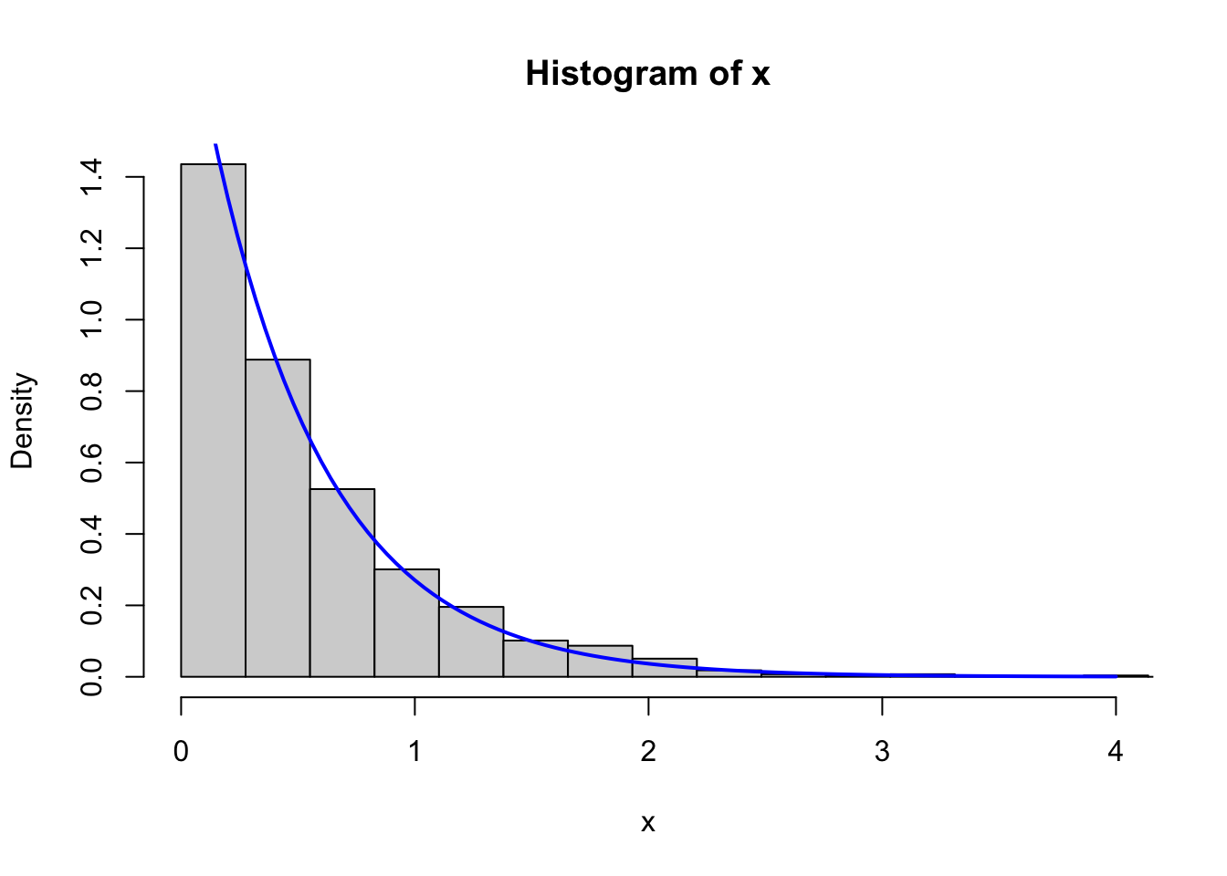
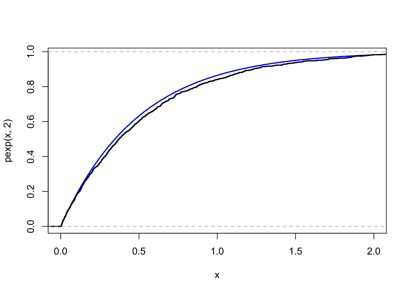
Figure 5.1: Left: Histogram of 1000 simulated data points from the exponential distribution with rate parameter \(\lambda = 2\) and the corresponding density. Right: The empirical (black) and theoretical (blue) distribution functions.
A curious detail is that if \(U\) is uniformly distributed on \((0, 1)\), then \(1 - U\) is uniformly distributed on \((0, 1)\). It is therefore possible to slightly simplify the implementation by replacing \(F^{-1}\) by \(- \log(u) / \lambda\), see Exercise 5.1.
Even if we do not have a simple analytic expression for the inverse distribution
function we might have an accurate approximation that is fast to evaluate,
which can then be used for simulation. An interesting example is the Gaussian
distribution. The call RNGkind() in the previous section revealed that the
default in
R
for generating samples from \(\mathcal{N}(0,1)\) is inversion. That is, Theorem
5.1 is used to transform uniform random
variables with the inverse distribution function \(\Phi^{-1}\). This function is,
however, non-standard, and R implements a technical
approximation
of \(\Phi^{-1}\) via rational functions.
Example 5.2 Another good example of a distribution that we can simulate by transformation is the \(t\)-distribution. Let \(Z = (Y, W) \in \mathbb{R} \times (0, \infty)\) with \(Y \sim \mathcal{N}(0, 1)\) and \(W \sim \chi^2_k\) independent.
Define \(T : \mathbb{R} \times (0, \infty) \to \mathbb{R}\) by \(T(y,w) = y / \sqrt{w/k},\) then
\[ X = T(Y, W) = \frac{Y}{\sqrt{W/k}} \]
has a \(t\)-distribution with \(k\) degress of freedom. Exercise 5.2 asks you to implement simulation from the \(t\)-distribution via the transformation above. This requires an algorithm that simulates from the Gaussian distribution and an algorithm that simulates from the \(\chi^2_k\) distribution (which is also a gamma distribution).
The R function rt() implements simulation from a \(t\)-distribution by the
above transformation and by generating \(W\) from a
gamma distribution with shape parameter \(k / 2\) and scale parameter \(2\).
The simulation from a gamma distribution via rejection sampling is
dealt with in Section 6.1.2.
5.3 Exercises
Exercise 5.1 Implement simulation from the exponential distribution as in Example
5.1 but replacing \(1 - U\) by \(U\). Test your
implementation and benchmark it against the implementation in
Example 5.1, against rexp() and
against dqrng::dqrexp() from the dqrng package.
Exercise 5.2 Implement simulation from the \(t\)-distribution as in Example
5.2. Test your
implementation and benchmark it against against rt().
Exercise 5.3 Recall that the Laplace distribution has density
\[ g(x) = \frac{1}{2} e^{-|x|} \]
for \(x \in \mathbb{R}\). Implement simulation from the Laplace distribution by transforming a uniform random variable by the inverse distribution function. Test the implementation
Exercise 5.4 If \(X\) and \(Y\) are independent and exponentially distributed with mean one, then \(X - Y\) has a Laplace distribution (why?). Use this to implement simulation from the Laplace distribution. Benchmark this implementation together with the implementation from Exercise ??.