A R programming
This appendix on R programming is a brief overview of important programming constructs and concepts in R that are used in the book. For a more extensive coverage of R as a programming language the reader is referred to the book Advanced R (Wickham 2019).
Depending on your background, the appendix can serve different purposes. If you already have experience with programming in R, this appendix can serve as a brush up on some basic aspects of the R language that are used throughout the book. If you have experience with programming in other languages than R, it can serve as an introduction to typical R programming techniques, where some may differ from what you know from other languages. If you have little prior experience with programming, this appendix can teach you the most important things for getting started with the book, but you are encouraged to follow up with additional and more detailed material like the book Advanced R.
Irrespective of your background, this appendix covers topics of greatest relevance for understanding how to implement correct and efficient numerical algorithms used in statistics. These topics are
- data types, comparisons and numerical precision
- functions and vectorized computations
- environments and function factories
- performance assessment and improvement
- S3 objects and methods
Several other topics of importance for R programming more broadly, such as S4 and R6 objects, expressions, and data wrangling, are not used much in the book and are not covered in any detail in this appendix. The reader is, in particular, referred to the book R for Data Science (2e) (Wickham, Çetinkaya-Rundel, and Grolemund 2023), for the use of R and Tidyverse as a framework for handling and visualizing data.
The book will not delve into questions regarding coding style either, but all code presented adheres to The tidyverse style guide unless there are specific reasons to deviate from it. The reader is encourage to adopt this style guide for their own code, or at least to make conscious and consistent decisions regarding any deviations.
A.1 Data structures
The fundamental data structure in R is a vector. Even variables that look and behave like single numbers are vectors of length one. Vectors come in two flavors: atomic vectors and lists.
An atomic vector is an indexed collection of data elements that are all of the same type, e.g.,
- integers
- floating-point numbers
- logical values
- character strings
A list is an indexed collection of elements without any type restrictions on the individual elements. An element in a list can, for instance, be a list itself.
A.1.1 Atomic vectors
You can construct a vector in R by simply typing in its elements, e.g.,
first_vector <- c(1, 2, 3)  # Note the 'c'
first_vector
## [1] 1 2 3The constructed vector contains the numbers 1, 2 and 3. We use the classical
assignment operator <- throughout, but R supports using the equal sign, =,
as the assignment operator if you prefer. The c() used on the right hand side
of the assignment is short for combine (or concatenate), and it is also used
if you combine two vectors into one.
## [1] 1 2 3 4 5 6There are several convenient techniques in R for constructing vectors of various
regular nature, e.g., sequences. The following example shows how to construct a
vector containing the integers from 1 to 10 using the colon operator. The type
of the resulting vector is integer indicating that the elements of the vector
are stored as integers.
integer_vector <- 1:10
integer_vector
## [1] 1 2 3 4 5 6 7 8 9 10
typeof(integer_vector) # 'typeof' reveals the internal storage mode## [1] "integer"We can access the individual elements as well as subsets of a vector by indices using square brackets.
integer_vector[3]## [1] 3
integer_vector[c(3, 4, 7)] # The 3rd, 4th and 7th elements## [1] 3 4 7The function seq() generalizes the colon operator as a way to generate regular
sequences. The following example shows how to generate a sequence,
double_vector, from 0.1 to 1.0 with increments of size 0.1. The type of the
resulting vector is double, which indicates that the elements of
double_vector are stored as doubles. That is, the numbers are stored as
floating-point numbers using 64 bits of storage for each number
corresponding to a precision of just about 16 digits.
double_vector <- seq(0.1, 1, by = 0.1)
double_vector
## [1] 0.1 0.2 0.3 0.4 0.5 0.6 0.7 0.8 0.9 1.0
typeof(double_vector)## [1] "double"Integers are often stored as or coerced into doubles automatically. The vectorfirst_vector appears to be an integer vector, but it is actually of type
double.
typeof(first_vector)## [1] "double"In R, numerical data of either type integer or double is collectively referred
to as numerics and have mode (and class) numeric. This may be confusing, in
particular because “numeric” is used also as pseudonym of the type double, but
it is rarely a practical problem. Doubles can be mixed with integers in any
computation, in which case the integers are automatically coerced to doubles. A
vector of numbers is therefore often said to by a numeric vector, irrespective
of whether the type is integer or double. Moreover, the function is.numeric()
tests if a vector is a numeric vector, and it returns TRUE for vectors of
type either double or integer.
It is possible to insist that integers are actually stored as integers by
appending L (capital l) to each integer, e.g.,
## [1] "integer"Apparent integers are usually—and silently—converted into doubles if they
are not explicitly marked as integers by L. One exception is when sequences
are generated using the colon operator with the endpoints being integers. The
result will then be a vector of type integer as was shown above with 1:10.
Vectors of any length can be created by the generic function vector(), or by
type specific functions such as numeric() that creates vectors of type double.
vector("numeric", length = 10)## [1] 0 0 0 0 0 0 0 0 0 0
numeric(10)## [1] 0 0 0 0 0 0 0 0 0 0Both vectors above are of type double and of length 10 and initialized with all elements being 0.
A logical vector is another example of a useful atomic vector. The default
type of a vector created by vector() is logical, with all elements being
FALSE.
vector(length = 10)## [1] FALSE FALSE FALSE FALSE FALSE FALSE FALSE FALSE FALSE FALSELogical vectors are encountered when we compare the elements of one vector to another vector or to a number.
logical_vector <- integer_vector > 4
logical_vector
## [1] FALSE FALSE FALSE FALSE TRUE TRUE TRUE TRUE TRUE TRUE
typeof(logical_vector)## [1] "logical"Note how the comparison above is vectorized, that is, each element in the
vector integer_vector is compared to the number 4 and the result is a vector
of logical values.
While a logical vector has its own type and is stored efficiently as such, it
behaves in many ways as a numeric vector with FALSE equivalent to 0 and TRUE
equivalent to 1. If we want to compute the relative frequency of elements in
integer_vector that are (strictly) larger than 4, say, we can simply take the
mean of logical_vector.
mean(logical_vector)## [1] 0.6Computing the mean of a logical vector works as if the logical values are coerced into zeros and ones before the mean is computed.
A final example of an atomic vector is a character vector. In this example, the vector is combined from 6 individual strings to form a vector of length 6. Combining strings into a vector does not paste the strings together—it forms a vector, whose elements are the individual strings.
character_vector <- c("A", "vector", "of", "length", 6, ".")
character_vector
## [1] "A" "vector" "of" "length" "6" "."
typeof(character_vector)## [1] "character"The type of the vector is character. Elements of a vector of type character are
strings. Note how the numeric value 6 in the construction of the vector was
automatically coerced into the string "6".
It is possible to paste together the strings in a character vector.
# Now a character vector of length 1
paste(character_vector, collapse = " ")
## [1] "A vector of length 6 ."It is likewise possible to split a string according to a pattern. For instance into its individual characters.
# Split the string "vector" into characters
strsplit(character_vector[2], split = "")
## [[1]]
## [1] "v" "e" "c" "t" "o" "r"Various additional string operations are available—see ?character for more
information.
In summary, atomic vectors are the primitive data structures used in R, with elements being accessible via indices (random access). Typical vectors contain numbers, logical values or strings. There is no declarations of data types—they are inferred from data or computations. This is a flexible type system with many operations in R silently coercing elements in a vector from one type to another.
A.1.2 Comparisons and numerical precision
We can compare vectors using the equality operator ==, which compares two
vectors element-by-element.
double_vector[2:3] == c(0.2, 0.3)## [1] TRUE FALSEThe result of the comparison above is a vector of length 2 containing the
logical values TRUE FALSE. If we recall the numbers contained in
double_vector the result might be surprising at first sight.
double_vector[2:3]## [1] 0.2 0.3The vector double_vector[2:3] appears to be equal to c(0.2, 0.3). The
difference shows up if we increase the number of printed digits from the default
(which is 7) to 20.
c(0.2, 0.3)## [1] 0.2000000000000000111 0.2999999999999999889
double_vector[2:3]## [1] 0.20000000000000001110 0.30000000000000004441The 0.3 produced by seq is computed as 0.1 + 0.1 + 0.1, while the 0.3 in the
vector c(0.2, 0.3) is converted directly into a double precision number. The
difference arises because neither 0.1 nor 0.3 are exactly representable in the
binary numeral system, and the arithmetic operations induce rounding errors. The
function numToBits can reveal the exact difference in the three least
significant bits.
numToBits(0.3)[1:3] # The three least significant bits## [1] 01 01 00
numToBits(0.1 + 0.1 + 0.1)[1:3]## [1] 00 00 01Differences in the least significant bits are tolerable when we do numerical computations but can be a nuisance for equality testing. When comparing vectors containing doubles we are therefore often interested in testing for approximate equality instead as illustrated by the following example.
test_vector <- c(0.1, 0.2, 0.3, 0.4, 0.5, 0.6, 0.7, 0.8, 0.9, 1.0)
all.equal(double_vector, test_vector)
## [1] TRUEThe function all.equal() has a tolerance argument controlling if numerical
differences will be regarded as actual differences. Another way of comparing
numerical vectors is by computing the range of their difference
range(double_vector - test_vector)## [1] 0.000000e+00 1.110223e-16This shows the largest positive and negative difference. Usually, the sizes of
the differences should be assessed relative to the magnitudes of the numbers
compared. For numbers approximately of magnitude 1, differences of the order
\(2^{-52} \approx 2.22 \times 10^{-16}\) (the “machine epsilon”) can safely be
regarded as rounding errors. The default (relative) tolerance of all.equal()
is the more permissive number \(\sqrt{2^{-53}} \approx 1.5 \times 10^{-8}\). This
number, the square root of the machine epsilon, is an ad hoc but commonly
used tolerance. See ?all.equal for details.
A.1.3 Lists
Recall that strsplit() with argument split = "" splits a string into its
individual characters. In fact, strsplit() returns a list with one entry for
each string in its first argument.
char_list <- strsplit(character_vector[2:4], split = "")
char_list
## [[1]]
## [1] "v" "e" "c" "t" "o" "r"
##
## [[2]]
## [1] "o" "f"
##
## [[3]]
## [1] "l" "e" "n" "g" "t" "h"The list char_list has length 3, with the first entry being a character vector
of length 6, the second entry a character vector of length 2 and the third entry
a character vector of length 6. A list just as a vector an indexed collection of
data entries, but a characteristic feature of a list is that the different
entries need not be of the same size or even the same type. In fact, each entry
of a list can be anything—even another list.
mixed_list <- list(c(1, 2), c(TRUE, FALSE))
combined_list <- list(mixed_list, char_list)
combined_list
## [[1]]
## [[1]][[1]]
## [1] 1 2
##
## [[1]][[2]]
## [1] TRUE FALSE
##
##
## [[2]]
## [[2]][[1]]
## [1] "v" "e" "c" "t" "o" "r"
##
## [[2]][[2]]
## [1] "o" "f"
##
## [[2]][[3]]
## [1] "l" "e" "n" "g" "t" "h"The list combined_list contains two lists, with the first list containing a
numeric and a logical vector, and with the second list containing character
vectors.
The different entries of a list can be accessed using indices in two different
ways—using either single brackets [] or double brackets [[]].
mixed_list[2]## [[1]]
## [1] TRUE FALSE
mixed_list[[2]]## [1] TRUE FALSEUsing only a single bracket will return a list containing the indexed elements of the full list, while the double bracket with a single index will return the element in the list with that index. The following demonstrates how to extract a specific entry in one of the vectors in the combined list.
combined_list[[2]][[1]][3] # Why does this return "c"?## [1] "c"Entries of atomic vectors as well as lists can be named, and an entry can be accessed via its name instead of its index. This may occasionally be useful for atomic vectors but is even more useful when working with lists. We reconstruct the combined list but with some descriptive names of its two entries.
combined_list <- list(mixed_bag = mixed_list, chars = char_list)We can then extract an entry of a list by its name—either via double brackets
or via the $ operator.
combined_list[["mixed_bag"]]## [[1]]
## [1] 1 2
##
## [[2]]
## [1] TRUE FALSE
combined_list$chars## [[1]]
## [1] "v" "e" "c" "t" "o" "r"
##
## [[2]]
## [1] "o" "f"
##
## [[3]]
## [1] "l" "e" "n" "g" "t" "h"One benefit of using names over numerical indices is that we do not need to keep track on the precise location of an entry within a list. This can make the code easier to read for humans, and code that uses names is robust to changes in the implementation of the precise location of the entry in the list.
The primary use of lists in this book is as a data structure for storing a small set of atomic vectors. We often need such a data structure when we write a function that needs to return more than just a single atomic vector. Thus lists are used as containers for function return values that are more complex than an atomic vector.
Lists can also be used as associative arrays that store key-value pairs, and where we can look up the value using the key. The key can then be of type character while the value can be anything. The lookup time is, however, linear in the length of the list. This can become a computational bottleneck for large lists, in which case it might be better to implement the associative array using environments. Environments can store key-value pairs just as lists, but they support faster lookup via a hash table, see Section A.2.2. They do, on the other hand, not support lookup via indices.
A.1.4 Other data structures
In addition to atomic vectors and lists any R programmer should know about the following three data structures:
- Factors
- Data frames
- Matrices and arrays
A factor is a special type of vector, whose entries are all from a fixed set of values (represented as strings) known as the factor levels. It is implemented as an integer vector with an attribute containing the factor levels—with the integers acting as pointers to the actual values stored in the attribute.
## [1] high low  low  low  high high
## Levels: high low
typeof(high_low)## [1] "integer"The factor above is initialized by a character vector, which is then converted into a factor. If the set of levels is small, a factor is more memory efficient than a naive implementation of a character vector. However, R actually stores character vectors via references to unique strings in a global string pool, so memory efficiency is not an argument for using a factor. Moreover, certain operations, such as concatenation, are more cumbersome for factors than for character vectors, and there is thus no reason to use factors unless some of their unique features are needed.
The main purpose of a factor is that it includes a specification of an ordering of the levels, which can differ from the alphabetic ordering. A number of R functions require factors, and in most cases it is because an ordering of the levels is needed. Factors should thus be used whenever we need the ordering or rely on other R functions that require us to use factors.
A data frame is R’s data structure for storing and handling tabular data. You can think of a data frame as a 2-dimensional table with rows and columns. All columns must be of the same length, and all entries in a single column are of the same type. A column is in practice often an atomic vector, but it does not need to.
combined_df <- data.frame(
  doubles = double_vector,
  integers = integer_vector,
  logicals = logical_vector
)
combined_df
## doubles integers logicals
## 1 0.1 1 FALSE
## 2 0.2 2 FALSE
## 3 0.3 3 FALSE
## 4 0.4 4 FALSE
## 5 0.5 5 TRUE
## 6 0.6 6 TRUE
## 7 0.7 7 TRUE
## 8 0.8 8 TRUE
## 9 0.9 9 TRUE
## 10 1.0 10 TRUEThe data frame constructed above has 10 rows and 3 columns. We can extract individual entries, rows, columns or rectangular parts of a data frame via brackets and indices.
combined_df[2, 2]## [1] 2
# Second row
combined_df[2, ]
## doubles integers logicals
## 2 0.2 2 FALSE
# Second column
combined_df[, 2]
## [1] 1 2 3 4 5 6 7 8 9 10
# Second and third row of columns two and three
combined_df[2:3, 2:3]
## integers logicals
## 2 2 FALSE
## 3 3 FALSEThe columns of a data frame have names, and we can extract a column by name in the same way as we can extract an entry in a list by name.
combined_df$logicals## [1] FALSE FALSE FALSE FALSE TRUE TRUE TRUE TRUE TRUE TRUEA data frame is, in fact, implemented as a list with each entry of the list storing one column of the data frame. It means that you can do everything with a data frame that you can do with a list.
Data frames play a very central role whenever we do data analysis or work with data in general—which is what statistics is ultimately about in practice. That aspect of statistics is, however, not very central to this book, and data frames only appear occasionally and are never part of the numerical algorithms that are otherwise in focus.
The last data structure covered in this section is arrays. A \(k\)-dimensional array can be thought of as a \(k\)-dimensional box of data, where we can access the entries of the box using \(k\) indices. If the dimensions of the array are \(n_1, n_2, \ldots, n_k\) the array is, in fact, just a length \(n_1 n_2 \cdots n_k\) vector with additional dimensionality attributes.
A matrix of dimensions \(n_1\) and \(n_2\) is a 2-dimensional array with \(n_1\) rows and \(n_2\) columns. We can access the entries of an array or a matrix using brackets with one index for each dimension of the array.
##      [,1] [,2]
## [1,]    1    3
## [2,]    2    4
mat[1, 2]## [1] 3
attributes(mat)## $dim
## [1] 2 2A matrix and a data frame appear similar. Both can be thought of as 2-dimensional arrays of data—but the similarity is superficial. We can extract entries and rectangular parts of matrices using brackets and indices, just as for data frames, but data frames allow for different data types in the different columns, and matrices do not. In fact, the intended usages of matrices and data frames are mostly different.
In contrast to data frames, matrices are used a lot in this book. For once, because a range of efficient numerical linear algebra algorithms are available for matrices and vectors, and many statistical computations can be reduced to numerical linear algebra.
A.2 Functions
When you write an R script and source it, the different R expressions in the script are evaluated sequentially. Intermediate results may be stored in variables and used further down in the script. It may not be obvious, but all the expressions in the script are, in fact, function calls. Your script relies on functions implemented in either core R packages or in other installed packages.
It is possible to use R as a scripting language without ever writing your own functions, but writing new R functions is how you extend the language, and it is how you modularize and reuse your code in an efficient way. As a first example, we implement the Gaussian kernel with bandwidth \(h\) (see also Section 2.1). The mathematical expression for this function is
\[ K_h(x) = \frac{1}{h \sqrt{2 \pi}} e^{- \frac{x^2}{2h^2}}, \]
which we usually think of as a collection of functions \(K_h : \mathbb{R} \to
[0,\infty)\) parametrized by \(h > 0\). Though \(x\) and \(h\) in this way play
different roles, they are treated equivalently in the implementation below,
where they are both arguments to the R function. We call the implemented
function gauss() to remind us that this is the Gaussian kernel.
The body of the function is the R expression
exp(- x^2 / (2 * h^2)) / (h * sqrt(2 * pi))
When the function is called with specific numeric values of its two formal
arguments x and h, the body is evaluated with the formal arguments replaced
by their values. The value of the (last) evaluated expression in the body is
returned by the function. The bandwidth argument h has a default value of 1,
so if h is not specified when the function is called, it gets the
value 1.
The Gaussian kernel with bandwidth \(h\) equals the density for the Gaussian
distribution with mean \(0\) and standard deviation \(h\). The dnorm() function
in R computes the Gaussian density, and we can thus compare
gauss() with dnorm().
## [1] 0.2419707 0.2419707## [1] 2.419707 2.419707For those two cases the functions appear to compute the same (at least, up to the printed precision).
Note how the formal argument sd is given the value 0.1 in the second call of
dnorm(). The argument sd is, in fact, the third argument of dnorm(), but
we do not need to specify the second, as in dnorm(0.1, 0, 0.1), to specify the
third. We can use its name instead, in which case the second argument in
dnorm() gets its default value 0.
There are several alternative ways to implement the Gaussian kernel that illustrate how functions can be written in R.
# A one-liner without curly brackets
gauss_one_liner <- function(x, h = 1)
  exp(- x^2 / (2 * h^2)) / (h * sqrt(2 * pi))

# A stepwise implementation computing the exponent first
gauss_step <- function(x, h = 1) {
  exponent <- x^2 / (2 * h^2)
  exp(- exponent) / (h * sqrt(2 * pi))
}

# A stepwise implementation with an explicit return statement
gauss_step_return <- function(x, h = 1) {
  exponent <- x^2 / (2 * h^2)
  value <- exp(- exponent) / (h * sqrt(2 * pi))
  return(value)
}
The following small test shows two cases where all implementations compute the same.
c(gauss(1), gauss_one_liner(1), gauss_step(1), gauss_step_return(1))## [1] 0.2419707 0.2419707 0.2419707 0.2419707
c(
  gauss(0.1, 0.1),
  gauss_one_liner(0.1, 0.1),
  gauss_step(0.1, 0.1),
  gauss_step_return(0.1, 0.1)
)
## [1] 2.419707 2.419707 2.419707 2.419707A function should always be tested. A test is a comparison of the return values
of the function with the expected values for some specific arguments. An
expected value can either be computed by hand or by another implementation— as
in the comparisons of gauss() and dnorm(). Such tests cannot prove that the
implementation is correct, but discrepancies can help you to catch and correct
bugs. Remember that when testing numerical computations that use floating-point
numbers we cannot expect exact equality. Thus tests should reveal if return
values are within an acceptable tolerance of the expected results.
Note that though the implementations of gauss_one_liner() and
gauss_step_return() are correct, they both violate the style guide. According
to the guide, curly braces should always be used when the function spans multiple
lines, and return() should only be used for early returns—not when the
function returns the last evaluated expression in the body. Whether we should
break (complicated) expressions into simpler pieces, as in gauss_step(), is a
judgment call, but see Section A.3 for how such a decision
affects the results from line profiling.
Larger pieces of software—such as an entire R package—should include a number of tests of each function it implements. This is known as unit testing (each unit, that is, each function, is tested), and there are packages supporting the systematic development of unit tests for R package development. A comprehensive set of unit tests also helps when functions are rewritten to, e.g., improve performance or extend functionality. If the rewritten function passes all tests, chances are that we did not break anything by rewriting the function.
It is good practice to write functions that do one well defined computation and to keep the body of a function relatively small. Then it is easier to reason about what the function does and it is easier to comprehensively test it. Complex behavior is achieved by composing small and well tested functions.
The overall aspects to writing an R function can be summarized as follows:
- A function has a name, it takes a number of arguments (possibly zero), and when called it evaluates its body and returns a value.
- The body is enclosed by curly brackets
{}, which may be left out if the body is only one line. - The function returns the value of the last expression in the body except when the body contains an explicit return statement.
- Formal arguments can be given default values when the function is implemented, and arguments can be passed to the function by position as well as by name.
- Functions should do a single well defined computation and be well tested.
A.2.1 Vectorization
In Section A.1 it was shown how comparison operators work in a vectorized way. In R, comparing a vector to another vector or a number leads to element-by-element comparisons with a logical vector as the result. This is one example of how many operations and function evaluations in R are natively vectorized, which means that when the function is evaluated with a vector argument the function body is effectively evaluated for each entry in the vector.
The gauss() function is another example of a function that automatically works
as a vectorized function.
## [1] 0.2419707 2.4197072It works as expected with vector arguments because all the functions in the body
of gauss() are vectorized, that is, the arithmetic operators are vectorized,
squaring is vectorized and the exponential function is vectorized.
It is good practice to write R programs that use vectorized computations whenever possible. The alternative is an explicit loop, which can be much slower. Several examples in the book illustrate the computational benefits of vectorized implementations. It may, however, not always be obvious how to implement a function so that it is correctly vectorized in all its arguments.
Suppose we want to implement the following function
\[ \overline{f}_h(x) = \frac{1}{N} \sum_{j=1}^N K_h(x - x_j) \]
for a dataset \(x_1, \ldots, x_N\) and with \(K_h\) the Gaussian kernel. This is the Gaussian kernel density estimator considered in Section 2.3. A straight forward implementation is
This implementation works correctly when x and h are single numbers but
when, e.g., x = c(0, 1) is a vector, the function does not return a vector but
a number apparently unrelated to \(\overline{f}_h(0)\) and \(\overline{f}_h(1)\).
c(f_bar(0, 1), f_bar(1, 1))## [1] 0.3128259 0.2154763
f_bar(c(0, 1), 1) # Computation is not vectorized, what happened?## [1] 0.2940242We leave it as an exercise for the reader to figure out which computation is
actually carried out when f_bar(c(0, 1), 1) is evaluated. A quick fix to make
any function correctly vectorized is the following explicit vectorization.
f_bar_vec <- Vectorize(f_bar)The R function Vectorize() takes a function as argument
and returns a vectorized version of it. That is, f_bar_vec() can be applied to
a vector, which results in applying f_bar() to each element of the vector. We
test that f_bar_vec() works correctly—both when the first and the second
argument is a vector.
f_bar_vec(c(0, 1), 1)## [1] 0.3128259 0.2154763
# Same result if we vectorize-by-hand
c(f_bar(0, 1), f_bar(1, 1))
## [1] 0.3128259 0.2154763
f_bar_vec(1, c(1, 0.1))## [1] 2.154763e-01 4.338004e-07
# Same result if we vectorize-by-hand
c(f_bar(1, 1), f_bar(1, 0.1))
## [1] 2.154763e-01 4.338004e-07The function Vectorize() is an example of a function
operator, which is a function
that takes a function as argument and returns a function. The function
Vectorize() basically wraps the computations of its argument function into a
loop, which applies the function to each element in the vector argument(s). For
prototyping and quick implementations it can be very convenient, but it is not
a shortcut to efficient vectorized computations.
Vectorize() is used in Section 2.3 to implement \(\overline{f}_h\)
based on dnorm(). The purpose of that implementation is to be able to compute
\(\overline{f}_h(x)\) for arbitrary \(x\) in a vectorized way. This is needed when
the function is plotted using curve() and in the likelihood computations of
that section. The implementations in Section 2.1.1 differ by
computing and returning
\[ \overline{f}_h(\tilde{x}_1), \ldots, \overline{f}_h(\tilde{x}_m) \]
for an equidistant grid \(\tilde{x}_1, \ldots, \tilde{x}_m\). That is, those implementations return the evaluations of \(\overline{f}_h\) in the grid and not the function \(\overline{f}_h\) itself.
A.2.2 Environments
Recall that in the implementation of f_bar() above, the body made use of the
variable xs, which is neither an argument to the function nor a variable
defined within the body. It may appear obvious that xs is supposed to refer to
the short data vector created just before the function implementation but
outside of the function. How does R know that?
Whenever the body of f_bar() is evaluated, R needs a procedure for looking up
the variable xs that appears in its body. Two possible procedures are:
- The variable is looked up as a local variable from wherever
f_bar()is called. - The variable is looked up as a local variable from wherever
f_bar()is defined.
To the user that calls f_bar() it might appear simpler if xs were looked
up from where the function is called. To the programmer that implements
f_bar() such a procedure will, however, make reasoning about the behavior of
f_bar() extremely difficult. The function f_bar() could be called from
anywhere or within any other function—even within a function that itself has a
variable called xs. So this is not how R works.
Computations implemented in the body of a function take place in a so-called evaluation environment, which is populated by variables defined in the body together with the arguments of the function (due to lazy evaluation of arguments, see Section A.2.3, this is technically a little imprecise). Whenever a variable is needed, which is not in the evaluation environment, it is looked up in the enclosing environment of the function. The default enclosing environment of any function is the environment where the function is defined.
environment(f_bar)## <environment: R_GlobalEnv>The function environment() returns the enclosing environment of f_bar(),
which in this case has a name and is R’s global environment—the place you
start in whenever you open R.
Environment is the technical term for a well defined “place” containing a collection of objects. When we write a computer program, environments constitute organizational components that allow different objects to have the same name—as long as they belong to different environments. When learning R we often start out by always implementing functions within the global environment and then we call functions from the global environment as well. For that reason it is easy to mistakenly believe that variables are looked up in the calling environment when, in fact, they are not. Or we might believe, equally wrongly, that variables are always looked up in the global environment. As described above, variables are always looked up in the enclosing environment of the function being evaluated, which just happens to be the global environment if the function is implemented in the global environment.
It is one thing to know the environment where a variable is looked up and
another to know the value of the variable. The following example demonstrates
that it is perfectly possible to change xs in the global environment between
calls of f_bar(), which will lead to different results.
f_bar(1, 1)## [1] 0.2154763
xs <- rnorm(10)
f_bar(1, 1)
## [1] 0.1927482Such behavior—that two calls of the same function with identical arguments
give different results—is often frowned upon, because it makes it difficult to
reason about what the function will do. When implementing a function in R it is
good practice to not rely on global variables like xs defined in the
global environment.
It is possible to construct and manipulate environments and, for instance, change the enclosing environment of a function.
environment(f_bar) <- new.env()
environment(f_bar)
## <environment: 0x3333c9bd8>The new environment is empty and its name is some obscure hexadecimal address.
Since it does not contain xs (yet) it is a good exercise to think about what
will happen if we call f_bar(1, 1) now? We leave the exercise to the reader
and populate the new environment with xs, evaluate f_bar(1, 1) and then we
change xs again in the global environment.
environment(f_bar)$xs <- xs
f_bar(1, 1)
## [1] 0.1927482
xs <- rnorm(10)
f_bar(1, 1)
## [1] 0.1927482Now f_bar() does not depend on the value of the global variable xs anymore.
It depends instead on its more private version of xs in its own enclosing
environment. In Section ?? we will systematize the
construction of functions having a private enclosing environment via function
factories. This is a good way of bundling a function with additional data
without relying on global variables.
The infrastructure of R also relies heavily on environments—it is environments that control how anything is found, variables as well as functions. Environments are, for instance, used to implement namespaces of packages that make it possible to load many packages without substantial conflicts due to functions having the same name in several packages. The stats namespace is an example of the environment containing all the functions implemented in the stats package.
asNamespace("stats")## <environment: namespace:stats>Despite the use of namespaces it happens occasionally that a function from one
package is masked by a function from another package. The package dplyr masks,
among other functions, the stats function filter(). When this happens we can
retrieve the function from the stats package’s namespace via
asNamespace("stats")$filter(), but the more convenient syntax for getting a
specific function from a namespace is stats::filter(). We can use the
double colon operator, ::, even when calling a function that is not masked. We
do so when the function is not implemented in a core R package to emphasize
which package actually implements the function—as a service to the reader.
As demonstrated in this section, environments are everywhere present when defining and calling functions and looking up variables. Moreover, if you need a hashed associative array, environments can do that for you, and they can thus be used as a data structure much like lists. It is, however, fairly uncommon to write R code as above that explicitly creates and assigns new environments let alone move data around between different environments. Most R programmers therefore rarely manipulate environments in your own code, but it is important to understand environments to be able to understand how R works and to reason correctly about how R functions look up other R functions and variables.
A.2.3 Function factories
The function Vectorize() introduced in Section A.2.1 is an
example of a function that returns a function. It is a general feature of the R
programming language that functions are just another data structure, which can
be defined and returned from within other functions. We can exploit this to
write constructor functions, whose purposes are to construct other functions
with private enclosing environments. We will refer to any such constructor
function as a
function factory. To
illustrate the idea we write a function factory that takes a dataset as argument
and returns the kernel density estimator as a function.
gauss_kernel_factory <- function(xs) {
  force(xs) # See explanation of this line below
  f_bar <- function(x, h) {
    mean(gauss(x - xs, h))
  }
  Vectorize(f_bar)
}
The function factory gauss_factory() defines the function f_bar() in its
body, which depends on the variable xs, and then returns a vectorized version
of f_bar(). The first line, force(xs), ensures that the value of the
argument xs is computed and stored when gauss_kernel_factory() is called.
When a function is called in R, its arguments are evaluated according to a
mechanism called lazy evaluation, which means that they
are not evaluated before they are actually needed. In the function factory
above, xs is not needed before the returned function is called, and unless we
force evaluation of xs we could be in for a surprise. The value of xs could
then change between the call of gauss_kernel_factory() and before its first
use, which is not desirable. Inserting the line force(xs) explicates that we
bypass the lazy evaluation to ensure that xs is what it was when
gauss_kernel_factory() was called.
Calling gauss_kernel_factory() with a specific data vector as argument will
construct an f_bar() for that data vector. We can compare with the previously
implemented vectorized f_bar_vec(), which relies on the global variable xs.
## [1] 0.2272297 0.4081006## [1] 0.2272297 0.4081006Since the global xs and the local xs in the environment of f_bar() are
identical, we get the same above whether we call f_bar() or f_bar_vec().
Changing the value of the global variable will not affect f_bar(), since it
contains a private copy of the data in its enclosing environment, while it does
affect f_bar_vec().
## [1] 0.2272297 0.4081006## [1] 0.2150577 1.3407070The function factory gauss_kernel_factory() illustrates a generally useful
idea in computational statistics. Oftentimes an R function will need both a
dataset and a number of additional arguments, but in a specific application the
dataset is fixed while the other arguments change. A kernel density estimator is
a prototypical example, while the likelihood function is another important
example. Alternatives to using a function factory is to either rely on a global
variable containing the data or to include data as an argument to the function.
The former is not recommended, and the latter makes the code more cluttered and
can be less efficient. Instead we can write a function factory that takes the
dataset as argument and returns a function of the other arguments. The function
factory can then include any preprocessing and transformations of the data that
might be needed, and these computations will only be carried out once when the
function factory is called.
A different usage of function factories is as a way to construct a cache for the function that the factory returns. If a function has a private enclosing environment we can safely use it to store values computed in one function call so that they can be retrieved in a subsequent call. We will illustrate caching by trying to solve an efficiency problem with generating random numbers sequentially in R.
Section 6.1.1 gives an implementation of a rejection sampler for the von
Mises distribution called vMsim_loop(), which relies on sequential generation
of two uniformly distributed random variables within a loop. In each iteration
there is a call of runif(1), which generates a single number from the uniform
distribution on \((0,1)\). As discussed in that section, this is slow. It is much
more efficient to call runif(1000) once than to call runif(1) a thousand
times, but the challenge is that in the rejection sampler we do not know upfront
how many uniform variables we need.
We solve this problem by implementing a function factory that returns a function, from which we can extract random numbers sequentially, but where the random number generator is called in a vectorized way and where the results are stored in the function’s enclosing environment, which then works as a cache.
runif_stream <- function(m, min = 0, max = 1) {
  cache <- runif(m, min, max)
  j <- 0
  function() {
    j <<- j + 1
    if (j > m) {
      cache <<- runif(m, min, max)
      j <<- 1
    }
    cache[j]
  }
}
The function factory above first initializes the cache to contain m samples
from the uniform distribution. It then returns a function for extracting random
numbers sequentially, which contains the cached samples in its enclosing
environment. The function generates a new vector of random variables whenever
the entire cache has been used. Note the use of the double headed assignment
operator <<-, which assigns to variables in the enclosing environment of the
function. Such assignments should usually only be done when the enclosing
environment is private to the function, e.g., when the function is constructed
by a function factory.
We will refer to the function returned by runif_stream() as a stream of
uniform random numbers, and we run a small test to check that a stream generates
samples from the uniform distribution in exactly the same way as if we generate
them sequentially using runif(1).
##  [1] 0.6905038 0.0623788 0.3614994 0.8189438 0.4347827 0.1792651 0.4446953
##  [8] 0.1601098 0.9025899 0.0501465
# Reset the seed and construct the stream with a cache of size 5
set.seed(3012)
runif_next <- runif_stream(5)
# The stream generates the same values
replicate(10, runif_next())
## [1] 0.6905038 0.0623788 0.3614994 0.8189438 0.4347827 0.1792651 0.4446953
## [8] 0.1601098 0.9025899 0.0501465It appears that the stream performs correctly, but it remains unclear if there is any point to using the stream. The next section will explore how to measure runtime and memory usage of small pieces of R code, which can be used for comparisons of different implementations.
A.3 Performance
Whenever we evaluate an R function it carries out some computations, which take a certain amount of time and require a certain amount of memory. The efficiency of an implementation is often assessed by its runtime and memory usage, and we need tools to be able to measure these quantities.
Ideally an implementation should be both fast and use as little memory as possible. There is, however, a tradeoff between time and memory consumption in the sense that we may be able to reduce runtime of an implementation at the price of increasing its memory usage or vice versa. It can be complicated to fully understand this tradeoff in practice, and it can also be problem specific whether memory usage or runtime is the most critical quantity to minimize. In this section we focus on how to measure these quantities in practice when we use R.
We will use the package bench, which contains several useful functions for high resolution measurements of time and for measuring memory usage of R computations. To measure memory usage, R needs to be compiled to support memory profiling, which is currently the case for the binary distributions for macOS and Windows.
The example below uses the mark() function from the bench package to collect
benchmark information on using either runif(1) or a uniform stream in a loop.
bench::mark(
  runif = for (i in 1:10000) runif(1),
  stream = {
    runif_next <- runif_stream(1000)
    for (i in 1:10000) runif_next()
  },
  check = FALSE,     # See explanation below
  filter_gc = FALSE  # See explanation below
)
## # A tibble: 2 × 6
## expression min median `itr/sec` mem_alloc `gc/sec`
## <bch:expr> <bch:tm> <bch:tm> <dbl> <bch:byt> <dbl>
## 1 runif 3.91ms 4.02ms 233. 11.1KB 5.99
## 2 stream 3.1ms 3.21ms 303. 122.8KB 1.99The results of the benchmark above shows that the median runtime for sequential
sampling is about 3 times larger when using runif() than if we use the stream.
The table also provides additional information, e.g., the total amount of memory
allocated.
The last column of output from the benchmark shows the number of garbage
collections per second during the benchmark. The gc refers to calls of the
garbage collector, which does the automatic memory
deallocation. That is, it is a function that detects memory allocated by R but
no longer in use and sets it free. You can call gc() to trigger garbage
collection and obtain information about memory allocated by R, but we usually
let R do this automatically. Even if the amount of memory used by an algorithm
is insignificant compared to the memory available, memory allocation and
deallocation take time and affect the runtime negatively. Implementations that
use little memory rarely trigger garbage collection and are therefore often
preferable.
Benchmarks are used throughout the book for measuring runtime (and memory
usage) of various implementations, and using bench::mark() to do so has
several advantages. First, it checks by default if the results from each
expression that we benchmark are equal. This is a good default since we should
only compare expressions that solve the same problem. This check does, however,
not make sense when simulating random numbers, and that is why the check was
disabled above. Second, bench::mark() randomizes and repeats the evaluations
of each expression, and the results are averages over the repeats. These
averages exclude by default iterations with garbage collection (set filter_gc = FALSE to change this). This is done to better separate time used on the actual
computations and time used on memory deallocation—but remember that both
matter in practice.
The bench package offers a few additional tools, e.g., automatic plotting of
benchmark results. For running benchmarks across a grid of parameter values, the
press() function is extremely useful. The package also includes
hires_time(), which returns high-resolution real time. We have used that
function in the package CSwR for implementing the tracer functionality covered
in Section A.3.2.
A.3.1 Profiling
While benchmarks can be useful for comparing the overall runtime of different implementations, they do not provide information about what goes on within the implementations. In particular, they do not tell us where the bottlenecks are in slow code. We need another tool for that, which is known as profiling. The R package profvis supports line profiling, which measures how much time was spent on each line of code within one or more functions during evaluation.
Running the following code will profile the implementation of the random number stream and store the result in as an interactive HTML widget. The widget can be shown either in RStudio or in the system browser.
p <- profvis::profvis(
{
runif_stream <- function(m, min = 0, max = 1) {
cache <- runif(m, min, max)
j <- 0
function() {
j <<- j + 1
if (j > m) {
cache <<- runif(m, min, max)
j <<- 1
}
cache[j]
}
}
runif_next <- runif_stream(1000)
for (i in 1:5e6) runif_next()
}
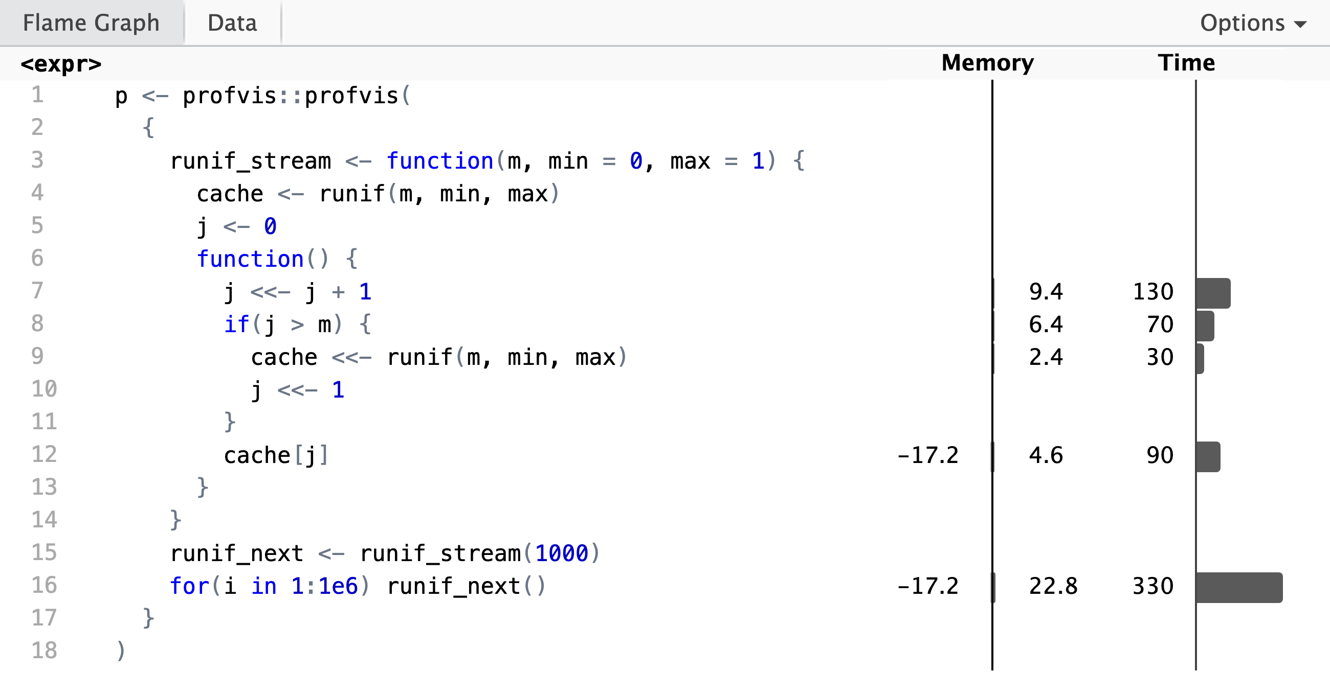
)A screenshot of the HTML widget is shown below. From this we see that obtaining
five million uniformly distributed numbers generated in batches of 1000 took
about 1500 ms in total, and we see how the time is distributed among the
different lines of code. The actual generation of the random numbers makes up
only about 10% of the total runtime—the rest of the time was spent on things
like incrementing the counter, j <<- j + 1, or extracting the \(j\)-th entry
from the cache, cache[j].
In addition to the visual summary above, the
interactive HTML widget shows the
data in the form of a flame graph, and it includes an alternative
summarized view of the profiling data. The profiling data itself is collected by
profvis() via the the Rprof() function from the utils
package. The main advantage of using profvis() is the way it processes and
formats the data—see ?Rprof to understand how the profiler actually works.
For profvis() to connect the profiling data to lines of code it must have
access to the source code. In the example above the source code of
runif_stream() was passed on to profvis() within a single R expression, but
it is also possible to profile the evaluation of a function without passing the
entire source code of that function as part of the expression. If
runif_stream() is implemented in a file, which is read into R via the
source() function (with option keep.source = TRUE), then calling
profvis(for(i in 1:1e6) runif_next()) will give us the same profiling data as
shown above. Note that the code has to be read from the file using source() and
not copy-pasted! Note also that for the profiler to provide meaningful data, the
total evaluation time has to be long enough. That is why we do a million
evaluations of runif_next() in a loop instead of just a single one.
To illustrate the use of the profiler with sourced code, we reconsider the different implementations of the Gaussian kernel from Section A.2.
source("scripts/gauss.R", keep.source = TRUE)
x <- rnorm(10000) # Test data
# Forcing JIT, see explanation below
gauss(x)
gauss_step(x)
gauss_step_alt(x)
The script gauss.R contains the implementation of three functions. The
gauss() and gauss_step() as in Section A.2 and then
gauss_step_alt(), which is similar to gauss_step() but with a small
reorganization of some arithmetic operations. After sourcing the script,
but before running the profiler, all functions are evaluated once. This is
done to trigger the just-in-time (JIT) compilation of the functions to byte code,
see ?compiler::enableJIT, and thus to avoid that this compilation step is
included in the profiling. We then run the profiler, in this case with
a large number of repeated calls of each function. This is to make the execution
time long enough for the profiler to be able to sample enough data.
p <- profvis::profvis( {
  for (i in 1:10000) gauss(x)
  for (i in 1:10000) gauss_step(x)
  for (i in 1:10000) gauss_step_alt(x)
}
)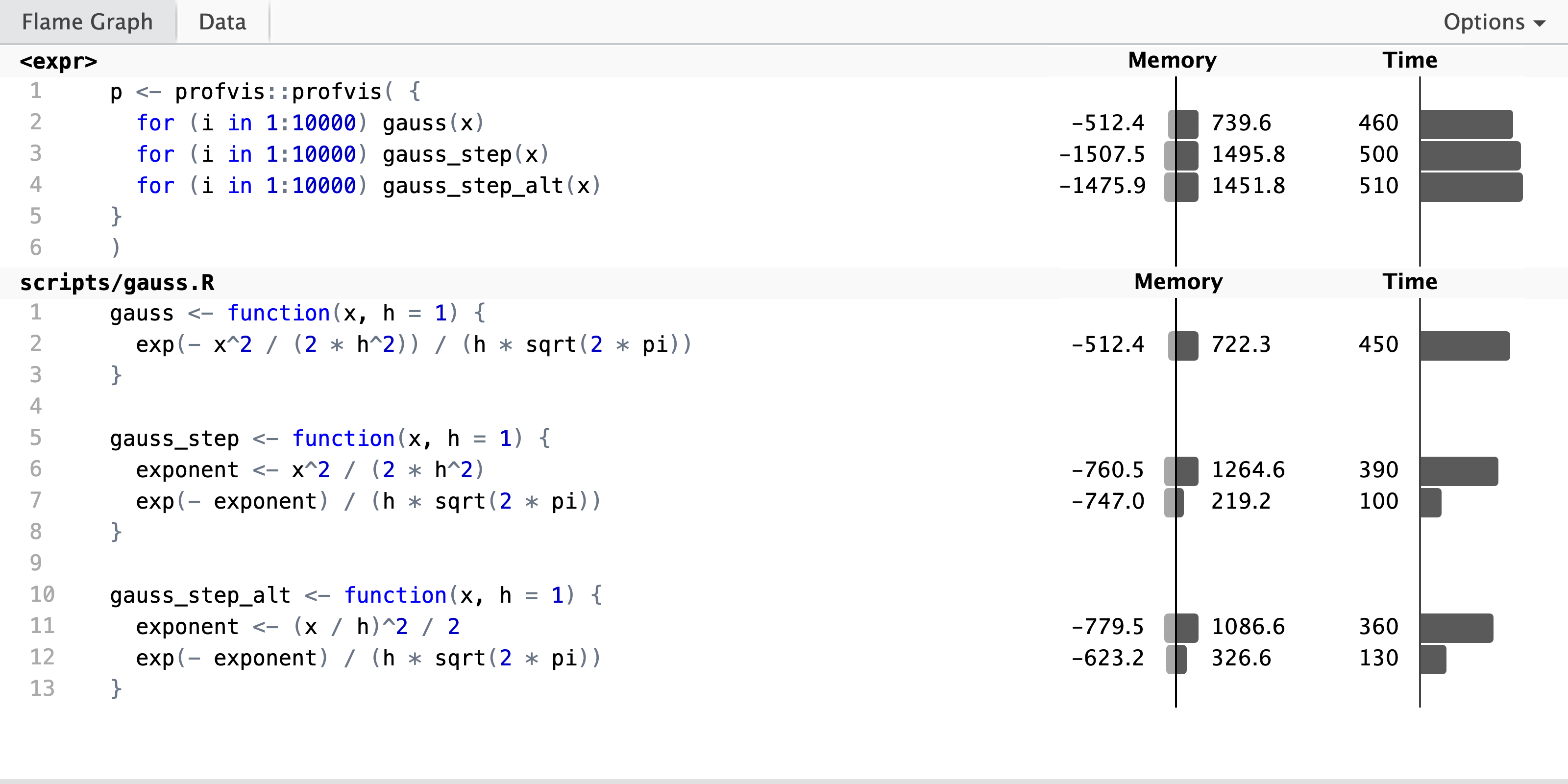
The profiling result shows that there is little difference between the three implementations in terms of runtime. The one-liner is a bit faster, probably because the step-wise solutions allocate and deallocate more memory due to the use of an extra temporary variable. From the perspective of line profiling, it is noteworthy that the two step-wise solutions give us more information about the runtime of the individual computations. Thus if you want to profile a complicated computation to understand how smaller parts of the computation affect runtime, you need to have each part of the computation on a separate line to get this information from line profiling tools.
A.3.2 Tracing
When R executes code, e.g., by evaluating a function we implemented ourselves, we would often like to peek into the interior of the function during evaluation and investigate what is going on. Besides curiosity there are two main reasons for why we want to do that. First, we might want to fix a bug. That is, when evaluating the function we get an error or a warning, or the function returns a value we know or suspect to be wrong. In those cases we need to debug the code to localize and fix the mistake(s). Second, we might want to track how a variable defined inside the body of the function evolves during the evaluation.
One pedestrian solution to the problem of peeking into a function while it is evaluated is to insert some additional code into the body of the function that can either print or store values of variables. That is, however, not a very efficient solution, and we need to remember to revert any changes we made, which can be a tedious and error-prone process.
Fortunately there are several good tools and techniques available for browsing
and tracing what is going on during a function evaluation. For once, R includes
debugging tools via the functions browser(), debug() and trace(), and
RStudio uses these to support debugging via visual breakpoints in the code and
it provides an interactive GUI session with access to the interior of a function
once a breakpoint is reached. We will not cover how these standard tools are used,
but they are highly recommended as much better alternatives to
debugging-by-print-statements.
What we will cover in some detail is a technique for tracing what is going on
during the evaluation of a function call, which can then be used for subsequent
analysis of the performance of an algorithm and its implementation. The
objective is to be able to store values of one or more variable from inside a
function during normal function evaluation without altering the implementation
of the function. We present a solution based on tracer objects,
created by the tracer() function, from the CSwR package. Using these
tracer objects we can
experiment with collecting any type of data during the function evaluation
without touching the implementation of the function or affecting its performance
when we are not tracing its behavior.
Using tracer objects with a function requires that we can call the object’s
tracer function inside the body of the function. It is possible to inject
such an function call into any function using the base R function trace(),
and to remove it again with the untrace() function. This can be done
programmatically, but it may be impossible to position the tracer call
at the right place this way, in which case we need to manually edit
the code. This is fine for interactive usage, but in this book we have taken a slightly different approach. All functions we need to trace are equipped with
a single so-called callback argument,
which effectively allows us to inject
and evaluate the tracer call at a particular position in the body of
the function.
To illustrate the use of tracer objects we implement a function computing the mean by a loop, which includes a callback argument.
mean_loop <- function(x, cb) {
  n <- length(x)
  x_sum <- 0
  for (i in seq_along(x)) {
    if (!missing(cb)) cb() # Callback
    x_sum <- x_sum + x[i]
  }
  x_sum / n
}
If any callback function is passed to mean_loop() via the cb argument
it is called in each iteration of the loop.
We proceed by constructing a tracer object with the tracer() function
from the CSwR package.
Its first argument is a vector of strings specifying the names of
the variables we want to trace. Below we will trace the cumulative sum
stored in x_sum. Its second argument, Delta, specifies how often the
tracer function prints trace information during evaluation.
Setting Delta = 0 means never. Finally, when calling mean_loop() we
pass the function mean_tracer$tracer() as the callback function.
mean_tracer <- CSwR::tracer("x_sum", Delta = 100)
x <- rnorm(1000)
x_bar <- mean_loop(x, cb = mean_tracer$tracer)
## n = 1: x_sum = 0;
## n = 100: x_sum = 12.71716;
## n = 200: x_sum = 5.742595;
## n = 300: x_sum = 10.00525;
## n = 400: x_sum = -3.001123;
## n = 500: x_sum = -22.21137;
## n = 600: x_sum = -16.96766;
## n = 700: x_sum = -13.71233;
## n = 800: x_sum = -24.16131;
## n = 900: x_sum = -18.22134;
## n = 1000: x_sum = -14.10883;With Delta = 100 the tracer prints out an iteration counter and the values of
the variables being traced every 100 iteration. The complete trace is stored
in the tracer object, and it can be inspected and analyzed by converting it to
a data frame using summary().
##         x_sum        .time
## 1  0.00000000 0.000000e+00
## 2 -0.88020663 1.024920e-06
## 3  0.07601509 1.639826e-06
## 4 -0.18070003 2.131797e-06
## 5  0.54705531 2.582790e-06
## 6  2.16323458 3.074994e-06
Included in the summary is the column .time, which contains the cumulative time
in seconds of each iteration. Some effort has gone into implementing the
timing of each iteration as accurately as possible. Time used by the tracer
itself is not included, and time spend on garbage collection is also excluded.
It is also possible to compute and trace additional variables not already in
the body of the function. This is done via the expr argument, which is given
a quoted expression. This expression is then evaluated in the context of the
functions body every time the tracer is called.
mean_tracer <- tracer(
  c("x_sum", "cum_mean"),
  Delta = 100,
  expr = quote(cum_mean <- x_sum / i)
)
x <- rnorm(1000)
x_bar <- mean_loop(x, cb = mean_tracer$tracer)
## n = 1: x_sum = 0; cum_mean = 0;
## n = 100: x_sum = -3.740253; cum_mean = -0.03740253;
## n = 200: x_sum = 15.57779; cum_mean = 0.07788893;
## n = 300: x_sum = 7.545286; cum_mean = 0.02515095;
## n = 400: x_sum = -11.07376; cum_mean = -0.02768441;
## n = 500: x_sum = -26.41054; cum_mean = -0.05282107;
## n = 600: x_sum = -32.58007; cum_mean = -0.05430012;
## n = 700: x_sum = -24.20555; cum_mean = -0.03457936;
## n = 800: x_sum = -18.63057; cum_mean = -0.02328821;
## n = 900: x_sum = -20.92425; cum_mean = -0.02324916;
## n = 1000: x_sum = -17.22585; cum_mean = -0.01722585;## x_sum cum_mean .time
## 1 0.00000000 0.000000000 0.000000e+00
## 2 -0.98614648 -0.493073240 1.230044e-06
## 3 -1.31704575 -0.439015251 1.886161e-06
## 4 -0.01576485 -0.003941213 2.419343e-06
## 5 -0.81594526 -0.163189051 2.952525e-06
## 6 -0.86963813 -0.144939688 3.485708e-06The summary above shows that we have now also traced the cumulative
mean of the \(x\)-s. It is possible to plot the traced variables
against runtime with the autoplot() function. The default is to
log-transform the time-axis, which is not what we want in this case.
The autoplot() function returns a standard ggplot object, which can
be modified as any other ggplot object. Here we add a horizontal
line at the total mean (x_bar).
autoplot(mean_tracer, cum_mean, log = FALSE) +
  geom_hline(yintercept = x_bar, color = "blue")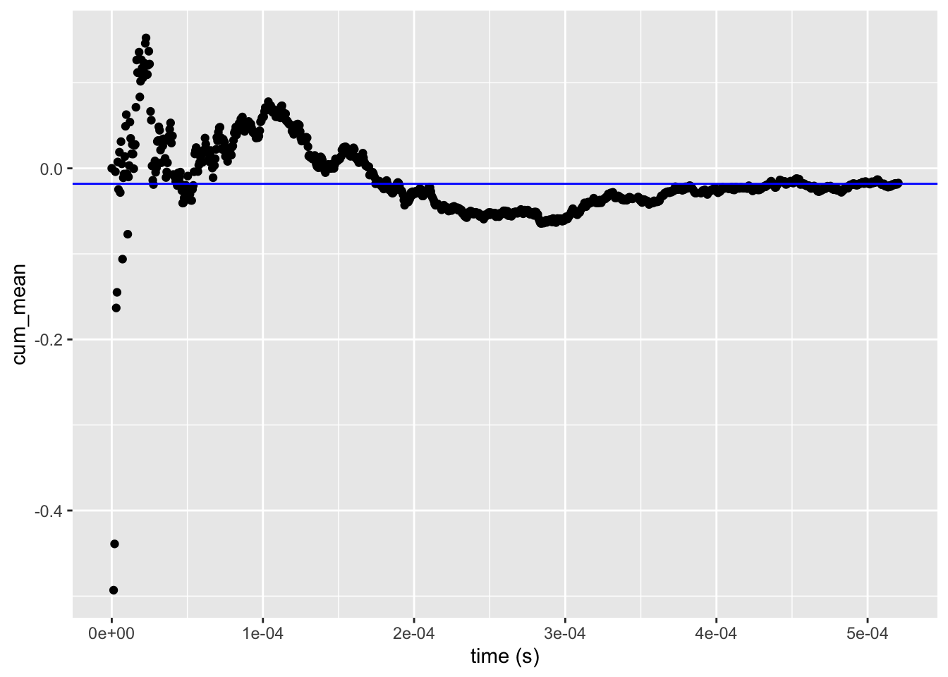
We can continue using the mean_tracer object for additional tracing, but the
information collected from earlier runs persists, and the new trace information
is just added to the object. We can, however, erase previous trace information
by calling a clear() function.
new_x <- rnorm(200)
# New trace information is added to any existing information.
x_bar <- mean_loop(new_x, cb = mean_tracer$tracer)
## n = 1100: x_sum = -3.124529; cum_mean = -0.03124529;
## n = 1200: x_sum = 1.611611; cum_mean = 0.008058055;
# Clearing the trace object makes it behave as if it was just created.
mean_tracer$clear()
x_bar <- mean_loop(new_x, cb = mean_tracer$tracer)
## n = 1: x_sum = 0; cum_mean = 0;
## n = 100: x_sum = -3.124529; cum_mean = -0.03124529;
## n = 200: x_sum = 1.611611; cum_mean = 0.008058055;For more information on using tracer() and tracer objects see ?CSwR::tracer.
Tracing is used throughout the book, but in particular in the chapters on
optimization. In Section A.4 we touch on the implementation of
tracer() as it relies on the S3 object system in R, and the implementation of
tracer() also uses environments extensively. The interested reader is
encouraged to study how tracer() is implemented for more insights on how
environments and function evaluation actually work in R.
A.3.3 Optimization of code
Knuth (1974) is famous for the quote “Premature optimization is the root of all evil”—with the keyword being premature. The point is that a programmer should not in the early development process worry about all sorts of possible but minor efficiency gains. In particularly not if such premature optimization leads to code that is more difficult to understand. Optimization is not premature once we have a working implementation and have identified the time or memory critical parts of the implementation. These are often minor parts of the implementation that are responsible for the majority of the runtime or memory usage. Once we have identified these parts using tools for benchmarking, profiling and tracing our code, we can begin to optimize the implementation of the critical parts.
- Dealt with throughout the book
- Mention parallel computations
A.5 Exercises
Functions
Exercise A.1 Explain the result of evaluating the following R expression.
(0.1 + 0.1 + 0.1) > 0.3## [1] TRUEExercise A.2 Write a function that takes a numeric vector x and a threshold value h
as arguments and returns the vector of all values in x greater than h.
Test the function on seq(0, 1, 0.1) with threshold 0.3. Have the example
from Exercise A.1 in mind.
Exercise A.3 Investigate how your function from Exercise A.2
treats missing values (NA), infinite values
(Inf and -Inf) and the special value “Not a Number” (NaN). Rewrite your
function (if necessary) to exclude all or some of such values from x.
Hint: The functions is.na, is.nan and is.finite are useful.
Histograms with non-equidistant breaks
The following three exercises will use a dataset consisting of measurements of infrared emissions from objects outside of our galaxy. We will focus on the variable F12, which is the total 12 micron band flux density.
infrared <- read.table("data/infrared.txt", header = TRUE)
F12 <- infrared$F12
The purpose of this exercise is two-fold. First, you will get familiar with the data and see how different choices of visualizations using histograms can affect your interpretation of the data. Second, you will learn more about how to write functions in R and gain a better understanding of how they work.
Exercise A.4 Plot a histogram of log(F12) using the default value of the argument breaks. Experiment with alternative values of breaks.
Exercise A.5 Write your own function, called my_breaks, which takes two arguments, x (a vector) and h (a positive integer). Let h have default value 5. The function should first sort
x into increasing order and then return the vector that: starts with the smallest entry in x;
contains every \(h\)th unique entry from the sorted x; ends with the largest entry in x.
For example, if h = 2 and x = c(1, 3, 2, 5, 10, 11, 1, 1, 3) the function should return c(1, 3, 10, 11). To see this, first sort x, which gives the vector c(1, 1, 1, 2, 3, 3, 5, 10, 11), whose unique
values are c(1, 2, 3, 5, 10, 11). Every second unique entry is c(1, 3, 10), and then the largest entry 11 is concatenated.
Hint: The functions sort and unique can be useful.
Use your function to construct breakpoints for the histogram for different values of h, and compare with the histograms obtained in Exercise A.4.
Exercise A.6 If there are no ties in the dataset, the function above will produce breakpoints
with h observations in the interval between two consecutive breakpoints
(except the last two perhaps). If there are ties, the function will by construction
return unique breakpoints, but there may be
more than h observations in some intervals.
The intention is now to rewrite my_breaks so that if possible each interval
contains h observations.
Modify the my_breaks function with this intention and so that is has the
following properties:
- All breakpoints must be unique.
- The range of the breakpoints must cover the range of
x. - For two subsequent breakpoints, \(a\) and \(b\), there must be at least
hobservations in the interval \((a,b],\) providedh < length(x). (With the exception that for the first two breakpoints, the interval is \([a,b].\))
Functions and objects
The following exercises build on having implemented a function that computes breakpoints for a histogram either as in Exercise A.5 or as in Exercise A.6.
Exercise A.7 Write a function called my_hist, which takes a single argument h and plots a
histogram of log(F12). Extend
the implementation so that any additional argument specified when calling my_hist
is passed on to hist. Investigate and explain what happens when executing
the following function calls.
my_hist()
my_hist(h = 5, freq = TRUE)
my_hist(h = 0)
Exercise A.8 Modify your my_hist function so that it returns an object of class my_histogram,
which is not plotted. Write a print method for objects of this class,
which prints just the number of cells.
Hint: It can be useful to know about the function cat.
How can you assign a class label to the returned object so that it is printed using your new print method, but it is still plotted as a histogram when given as argument to plot?
Exercise A.9 Write a summary method that returns a data frame with two columns containing the midpoints of the cells and the counts.
Exercise A.10 Write a new plot method for objects of class my_histogram that uses ggplot2 for plotting the histogram.
Functions and environments
The following exercises assume that you have implemented a my_hist function as in Exercise A.7.
Exercise A.11 What happens if you remove that data and call my_hist subsequently?
What is the environment of my_hist? Change it to a new environment, and assign
(using the function assign) the data to a
variable with an appropriate name in that environment. Once this is done,
check what now happens when calling my_hist after
the data is removed from the global environment.
Exercise A.12 Write a function that takes an argument x (the data) and
returns a function, where the returned function
takes an argument h (just as my_hist) and plots a histogram (just as my_hist).
Because the return value is a function, we may refer to the function
as a function factory.
What is the environment of the function created by the function factory? What is in the environment? Does it have any effect when calling the function whether the data is altered or removed from the global environment?
Exercise A.13 Evaluate the following function call:
tmp <- my_hist(10, plot = FALSE)What is the type and class of tmp? What happens when plot(tmp, col = "red")
is executed? How can you find help on what plot() does with an object of this
class? Specifically, how do you find the documentation for the argument col,
which is not an argument of plot()?