10 Expectation maximization algorithms
Somewhat surprisingly, it is possible to develop an algorithm, known as the expectation-maximization (EM) algorithm, for computing the maximum-likelihood estimate in situations where computing the likelihood itself is quite difficult. This is possible in situations where the model is defined in terms of certain unobserved components, and where likelihood computations and optimization is relatively easy had we observed everything. The EM algorithm exploits this special structure, and is thus not a general optimization algorithm, but it applies to commonly occurring problems in statistics, and it is one of the core optimization algorithms used for likelihood optimization.
In this chapter it is shown that the algorithm is generally an descent algorithm of the negative log-likelihood, and examples of its implementation are given to multinomial cell collapsing and Gaussian mixtures. The theoretical results needed for the EM algorithm for a special case of mixed models are given as well. Finally, some theoretical results as well as practical implementations for computing estimates of the Fisher information are presented.
10.1 Basic properties
In this section the EM algorithm is formulated and shown to be a descent algorithm for the negative log-likelihood. Allele frequency estimation for the peppered moth is considered as a simple example illustrating the implementation and application of the EM algorithm.
10.1.1 Incomplete data likelihood
Let \(X\) be a random variable and suppose that we observe \(Y = M(X)\). An example of this is given by collapsing of categories in the multinomial distribution as treated in Section 8.2.1. We assume that \(X\) has density \(f(\cdot \mid \theta)\) and that \(Y\) has marginal density \(g(\cdot \mid \theta)\).
The marginal density is typically of the form
\[ g(y \mid \theta) = \int_{\{x: M(x) = y\}} f(x \mid \theta) \ \mu_y(\mathrm{d} x) \]
for a suitable measure \(\mu_y\) depending on \(M\) and \(y\) but not \(\theta\). This general formula for the marginal density can often be derived from the coarea formula, see (Evans and Gariepy 2015), in particular their change-of-variable formula in Theorem 3.11.
The log-likelihood for observing \(Y = y\) is
\[ \ell(\theta) = \log g(y \mid \theta). \]
The log-likelihood is often impossible to compute analytically and difficult and expensive to compute numerically. The complete log-likelihood, \(\log f(x \mid \theta)\), is often easy to compute, but we do not observe \(X\), only that \(M(X) = y\).
In some cases it is possible to compute
\[ Q(\theta \mid \theta') := E_{\theta'}(\log f(X \mid \theta) \mid Y = y), \]
which is the conditional expectation of the complete log-likelihood given the observed data and computed using the probability measure given by \(\theta'\). Thus for fixed \(\theta'\) this is a computable function of \(\theta\) depending only on the observed data \(y\).
We could then get the following idea: with an initial guess of \(\theta' = \theta_0\) compute iteratively
\[ \theta_{n + 1} = \argmax_{\theta} \ Q(\theta \mid \theta_n) \]
for \(n = 0, 1, 2, \ldots\). This idea is the EM algorithm:
- E-step: Compute the conditional expectation \(Q(\theta \mid \theta_n )\).
- M-step: Maximize \(\theta \mapsto Q(\theta \mid \theta_n )\).
It is a bit weird to present the algorithm as a two-step algorithm in its abstract formulation. Even though we can regard \(Q(\theta \mid \theta_n)\) as something we can compute abstractly for each \(\theta\) for a given \(\theta_n\), the maximization is in practice not really done using all these evaluations. It is computed either by an analytic formula involving \(y\) and \(\theta_n\), or by a numerical algorithm that computes certain evaluations of \(Q( \cdot \mid \theta_n)\) and perhaps its gradient and Hessian. In computing these specific evaluations there is, of course, a need for the computation of conditional expectations, but we would compute these as they are needed and not upfront.
However, in some of the most important applications of the EM algorithm, we can quite often regard the algorithm as a two-step algorithm. This is the case whenever \(Q(\theta \mid \theta_n) = q(\theta, t(y, \theta_n))\) is given in terms of \(\theta\) and a function \(t(y, \theta_n )\) of \(y\) and \(\theta_n\) that does not depend on \(\theta\). Then the E-step becomes the computation of \(t(y, \theta_n )\), and in the M-step, \(Q(\cdot \mid \theta_n )\) is maximized by maximizing \(q(\cdot, t(y, \theta_n ))\). In this case the maximizer \(\theta_{n+1}\) becomes a function of \(t(y, \theta_n)\).
10.1.2 Monotonicity of the EM algorithm
We prove below that the algorithm (weakly) increases the log-likelihood in every step, and thus is a descent algorithm for the negative log-likelihood \(H = - \ell\).
It holds in great generality that the conditional distribution of \(X\) given \(Y = y\) has density
\[\begin{equation} h(x \mid y, \theta) = \frac{f(x \mid \theta)}{g(y \mid \theta)} \tag{10.1} \end{equation}\]
w.r.t. the measure \(\mu_y\) as above (that does not depend upon \(\theta\)), and where \(g\) is the density for the marginal distribution.
This can be verified quite easily for discrete distributions and when \(X = (Y, Z)\) with joint density w.r.t. a product measure \(\nu \otimes \mu\) that does not depend upon \(\theta\). In the latter case, \(f(x \mid \theta) = f(y, z \mid \theta)\) and
\[ g(y \mid \theta) = \int f(y, z \mid \theta) \ \mu(\mathrm{d} z) \]
is the marginal density w.r.t. \(\nu\). The conditional density
\[ h(y, z \mid \theta) = \frac{f(y,z \mid \theta)}{g(y \mid \theta)} \]
is w.r.t. \(\mu_y = \delta_y \otimes \mu\).
Whenever (10.1) holds it follows that
\[ \ell(\theta) = \log g(y \mid \theta) = \log f(x \mid \theta) - \log h(x \mid y, \theta), \]
where \(\ell(\theta)\) is the log-likelihood.
Theorem 10.1 If \(\log f(X \mid \theta)\) as well as \(\log h(X \mid Y, \theta)\) have finite \(\theta'\)-conditional expectation given \(M(Y) = x\) then
\[ Q(\theta \mid \theta') > Q(\theta' \mid \theta') \quad \Rightarrow \quad \ell(\theta) > \ell(\theta'). \]
Proof. Since \(\ell(\theta)\) depends on \(x\) only through \(y = M(x)\),
\[\begin{align*} \ell(\theta) & = \E_{\theta'} ( \ell(\theta) \mid Y = y) \\ & = \underbrace{\E_{\theta'} ( \log f(X \mid \theta) \mid Y = u)}_{Q(\theta \mid \theta')} + \underbrace{ \E_{\theta'} ( - \log h(X \mid y, \theta) \mid Y = y)}_{H(\theta \mid \theta')} \\ & = Q(\theta \mid \theta') + H(\theta \mid \theta'). \end{align*}\]
For the second term we find, using the elementary logarithmic inequality \(-\log(a) \geq 1 - a\) for \(a > 0\), that
\[\begin{align*} H(\theta \mid \theta') & = \int - \log(h(x \mid y, \theta)) h(x \mid y, \theta') \mu_y(\mathrm{d}x) \\ & = \int - \log\left(\frac{h(x \mid y, \theta)}{ h(x \mid y, \theta')}\right) h(x \mid y, \theta') \mu_y(\mathrm{d}x) \\ & \quad + \int - \log(h(x \mid y, \theta')) h(x \mid y, \theta') \mu_y(\mathrm{d}x) \\ & \geq \underbrace{\int h(x \mid y, \theta') \mu_y(\mathrm{d}x)}_{=1} - \int \frac{h(x \mid y, \theta)}{ h(x \mid y, \theta')} h(x \mid y, \theta') \mu_y(\mathrm{d}x) \\ & \quad + H(\theta' \mid \theta') \\ & = 1 - \underbrace{ \int h(x \mid y, \theta) \mu_y(\mathrm{d}x)}_{=1} + H(\theta' \mid \theta') \\ & = H(\theta' \mid \theta'). \end{align*}\]
From this we see that
\[ \ell(\theta) \geq Q(\theta \mid \theta') + H(\theta' \mid \theta') \]
for all \(\theta\). Observing that
\[ \ell(\theta') = Q(\theta' \mid \theta') + H(\theta' \mid \theta') \]
completes the proof of the theorem.
The proof above uses the inequality \(-\log(a) \geq 1 - a\), which is, e.g., a consequence of \(a \mapsto -\log(a)\) being a convex function. It is possible to use Jensen’s inequality instead. Alternatively, we could refer to Gibbs’ inequality in information theory stating that the Kullback-Leibler divergence is positive, or equivalently that the cross-entropy \(H(\theta \mid \theta')\) is smaller than the entropy \(H(\theta' \mid \theta')\). The proofs of those inequalities are themselves consequences of \(a \mapsto -\log(a)\) being convex, and using the elementary inequality \(-\log(a) \geq 1 - a\) is the most direct way to show Theorem 10.1. It is worth noting that there is equality if and only if \(a = 1\), which implies that \(Q(\theta \mid \theta') > Q(\theta' \mid \theta')\) unless the \(\theta\)-conditional distribution of \(X \mid Y = y\) is the same as the \(\theta'\)-conditional distribution.
It follows from Theorem 10.1 that if \(\theta_n\) is computed iteratively starting from \(\theta_0\) such that
\[ Q(\theta_{n+1} \mid \theta_{n}) > Q(\theta_{n} \mid \theta_{n}), \]
then \[ H(\theta_0) > H(\theta_1) > H(\theta_2) > \ldots. \]
This proves that the EM algorithm is a strict descent algorithm for the negative log-likelihood as long as it is possible in each iteration to find a \(\theta\) such that \(Q(\theta \mid \theta_{n}) > Q(\theta_{n} \mid \theta_{n}).\)
The term EM algorithm is reserved for the specific algorithm that maximizes \(Q(\cdot \mid \theta_n)\) in the M-step, but there is no reason to insist on the M-step being a maximization. A choice of ascent direction of \(Q(\cdot \mid \theta_n)\) and a step-length guaranteeing sufficient descent of \(H\) (sufficient ascent of \(Q(\cdot \mid \theta_n)\)) will be enough to give a descent algorithm. Any such variation is usually termed a generalized EM algorithm.
The lower bound \(Q(\theta \mid \theta') + H(\theta' \mid \theta')\) of the log-likelihood, as derived in the proof above, is sometimes called a minorant for the log-likelihood. The EM algorithm can thus be seen as alternating between maximizing a minorant (M-step) and updating the minorant (E-step). We could imagine that the minorant is a useful lower bound on the difficult-to-compute log-likelihood. The additive constant \(H(\theta' \mid \theta')\) in the minorant is, however, not computable in general either, and it is not clear that the bound can be used quantitatively.
We implement a generic version of the EM algorithm below via
a function factory. The function factory returns a function that iteratively
computes the composition of an E-step and an M-step using
problem specific implementations of these steps. These are passed as
arguments to the function factory. The algorithm stops when the
relative change of the parameter values is sufficiently small, cf.
Section 9.2.3, and it is controlled by the tolerance
argument epsilon, which is given the default value \(10^{-6}\) by
the function factory if not specified.
em_factory <- function(e_step, m_step, eps = 1e-6) {
  force(e_step); force(m_step); force(eps)
  function(par, y, epsilon = eps, cb = NULL, ...) {
    repeat {
      par0 <- par
      par <- m_step(e_step(par, y, ...), y, ...)
      if (!is.null(cb)) cb()
      if (sum((par - par0)^2) <= epsilon * (sum(par^2) + epsilon))
        break
    }
    par  # Returns the parameter estimate
  }
}
The function returned by em_factory() has the callback argument, cb,
and any additional arguments are, via ..., passed on to both
the E-step and the M-step.
10.1.3 Peppered moths
We return in this section to the peppered moths and the implementation of the EM algorithm for multinomial cell collapsing. We recall the implementation of the multinomial collapsing map.
The EM algorithm can be implemented by two simple functions that compute conditional expectations (the E-step) and the maximization of the complete observation log-likelihood, respectively.
e_step_mult <- function(p, ny, group, ...) {
  ny[group] * p / mult_collapse(p, group)[group]
}
The MLE of the complete log-likelihood is a linear estimator, as is the case in many examples with explicit MLEs.
The e_step_mult() and m_step_mult() functions are abstract implementations. They require specification of the arguments group and X, respectively, to become concrete. The M-step is also only implemented in the case where the
complete-data maximum-likelihood estimator is a
linear estimator, that is, a linear map of the complete data vector \(ny\)
that can be expressed in terms of a matrix \(\mathbf{X}\).
To implement problem specific versions of these functions for the peppered
moth model we need the mapping from the parameter space to the vector
of genotype probabilities, and we need the specific matrix X for computing
the linear estimator.
prob_pep <- function(p) {
  p[3] <- 1 - p[1] - p[2]

  out_of_bounds <-
    p[1] > 1 || p[1] < 0 || p[2] > 1 || p[2] < 0 || p[3] < 0
  if (out_of_bounds) return(NULL)

  c(p[1]^2, 2 * p[1] * p[2], 2 * p[1] * p[3],
    p[2]^2, 2 * p[2] * p[3], p[3]^2
  )
}

X_pep <- matrix(
  c(2, 1, 1, 0, 0, 0,
    0, 1, 0, 2, 1, 0) / 2,
  2, 6, byrow = TRUE
)

e_step_pep <- function(par, ny, ...) {
  e_step_mult(prob_pep(par), ny, c(1, 1, 1, 2, 2, 3), ...)
}

m_step_pep <- function(ny, ...) {
  m_step_mult(ny, X_pep, ...)
}
The EM algorithm for the peppered moth model is finally obtained by calling em_factory() with arguments e_step_pep() and m_step_pep(). The resulting
function can then be applied to the data with some starting point, and it will
compute the maximum-likelihood estimator.
em_pep <- em_factory(e_step_pep, m_step_pep)## [1] 0.07084 0.18877We check what is going on in each step of the EM algorithm.
## n = 1: par = 0.08039, 0.22464;
## n = 2: par = 0.07119, 0.19547;
## n = 3: par = 0.07085, 0.18993;
## n = 4: par = 0.07084, 0.18895;
## n = 5: par = 0.07084, 0.18877;
## [1] 0.07084 0.18877
em_tracer <- CSwR::tracer(c("par0", "par"), Delta = 0)
phat_pep <- em_pep(c(0.3, 0.3), c(85, 196, 341),
  epsilon = 1e-20,
  cb = em_tracer$tracer
)
em_trace <- summary(em_tracer)
em_trace <- transform(
  em_trace,
  n = seq_len(nrow(em_trace)),
  par_norm_diff = sqrt((par0.1 - par.1)^2 + (par0.2 - par.2)^2)
)
ggplot(em_trace, aes(n, par_norm_diff)) +
  geom_point() +
  scale_y_log10()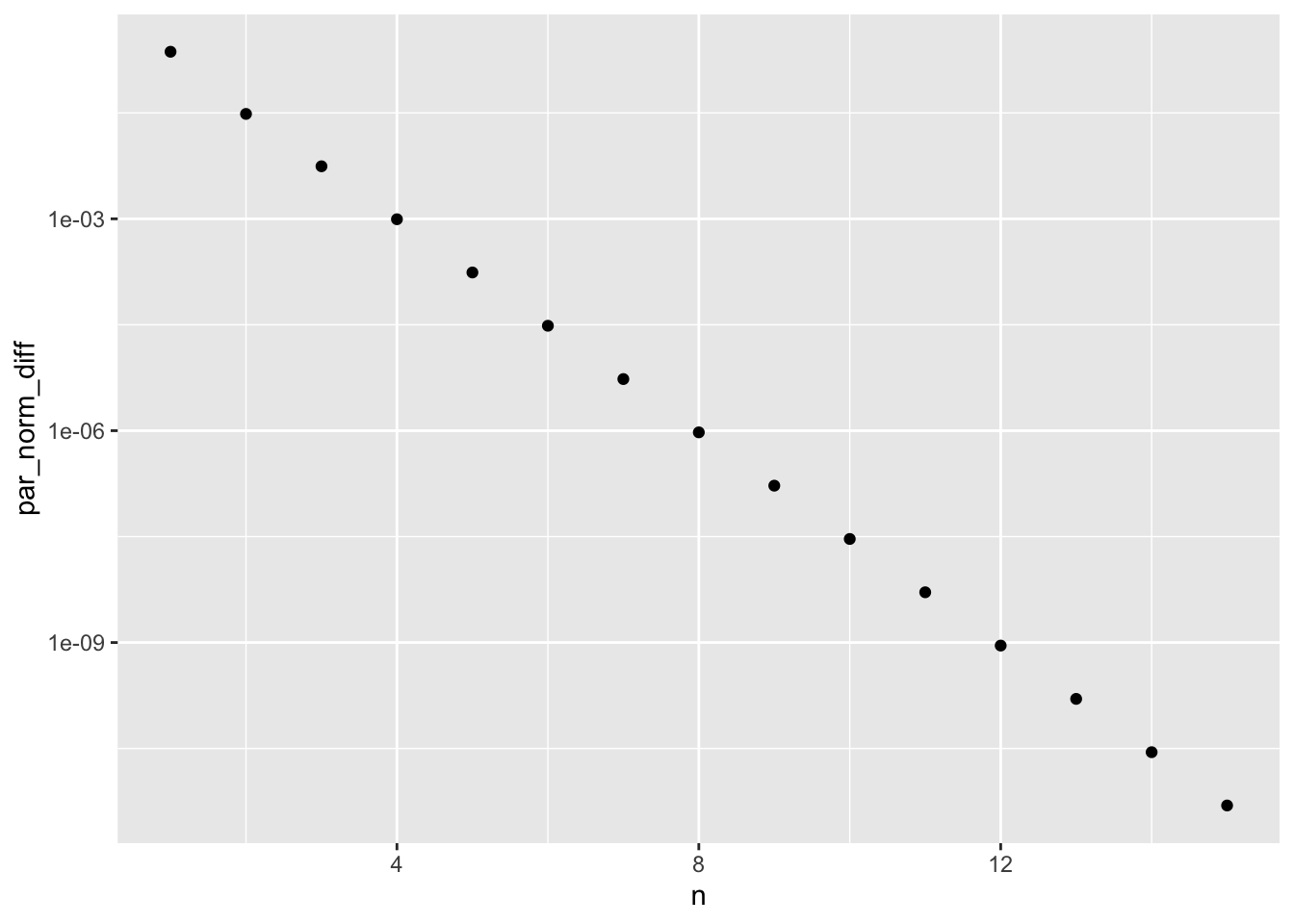
Note the log-axis. The EM algorithm converges linearly (this is the terminology, see Algorithms and Convergence). The log-rate of the convergence can be estimated by least-squares.
log_rate_fit <- lm(log(par_norm_diff) ~ n,  data = em_trace)
exp(coefficients(log_rate_fit)["n"])
## n
## 0.175The rate is very small in this case implying fast convergence. This is not always the case. If the log-likelihood is flat, the EM algorithm can become quite slow with a rate close to 1.
10.2 Exponential families
We consider in this section the special case where the model of \(\mathbf{y}\) is given as an exponential family Bayesian network and \(x = M(\mathbf{y})\) is the observed transformation.
The complete data log-likelihood is \[\theta \mapsto \theta^T t(\mathbf{y}) - \kappa(\theta) = \theta^T \sum_{j=1}^m t_j(y_j) - \kappa(\theta),\] and we find that \[Q(\theta \mid \theta') = \theta^T \sum_{j=1}^m E_{\theta'}(t_j(Y_j) \mid X = x) - E_{\theta'}( \kappa(\theta) \mid X = x).\]
To maximize \(Q\) we differentiate \(Q\) and equate the derivative equal to zero. We find that the resulting equation is \[\sum_{j=1}^m E_{\theta'}(t_j(Y_j) \mid X = x) = E_{\theta'}( \nabla \kappa(\theta) \mid X = x).\]
Alternatively, one may also note the following general equation for finding the maximum of \(Q(\cdot \mid \theta')\) \[\sum_{j=1}^m E_{\theta'}(t_j(Y_j) \mid X = x) = \sum_{j=1}^m E_{\theta'}(E_{\theta}(t_j(Y_j) \mid y_1, \ldots, y_{j-1}) \mid X = x),\] since \[E_{\theta'}(\nabla \kappa(\theta)\mid X = x) = \sum_{j=1}^m E_{\theta'}(\nabla \log \varphi_j(\theta) \mid X = x) = \sum_{j=1}^m E_{\theta'}(E_{\theta}(t_j(Y_j) \mid y_1, \ldots, y_{j-1}) \mid X = x) \]
Example 10.1 Continuing Example 8.5 with \(M\) the projection map
\[ (\mathbf{y}, \mathbf{z}) \mapsto \mathbf{y} \]
we see that \(Q\) is maximized in \(\theta\) by solving
\[ \sum_{i,j} E_{\theta'}(t(Y_{ij} \mid Z_i) \mid \mathbf{Y} = \mathbf{y}) = \sum_{i} m_i E_{\theta'}(\nabla \kappa(\theta \mid Z_i) \mid \mathbf{Y} = \mathbf{y}). \]
By using Example 8.3 we see that
\[ \kappa(\theta \mid Z_i) = \frac{(\theta_1 + \theta_3 Z_i)^2}{4\theta_2} - \frac{1}{2}\log \theta_2, \]
hence
\[ \nabla \kappa(\theta \mid Z_i) = \frac{1}{2\theta_2} \left(\begin{array}{cc} \theta_1 + \theta_3 Z_i \\ - \frac{(\theta_1 + \theta_3 Z_i)^2}{2\theta_2} - 1 \\ \theta_1 Z_i + \theta_3 Z_i^2 \end{array}\right) = \left(\begin{array}{cc} \beta_0 + \nu Z_i \\ - (\beta_0 + \nu Z_i)^2 - \sigma^2 \\ \beta_0 Z_i + \nu Z_i^2 \end{array}\right). \]
Therefore, \(Q\) is maximized by solving the equation
\[ \sum_{i,j} \left(\begin{array}{cc} y_{ij} \\ - y_{ij}^2 \\ E_{\theta'}(Z_i \mid \mathbf{Y} = \mathbf{y}) y_{ij} \end{array}\right) = \sum_{i} m_i \left(\begin{array}{cc} \beta_0 + \nu E_{\theta'}(Z_i \mid \mathbf{Y}_i = \mathbf{y}_i) \\ - E_{\theta'}((\beta_0 + \nu Z_i)^2 \mid \mathbf{Y} = \mathbf{y}) - \sigma^2 \\ \beta_0 E_{\theta'}(Z_i \mid \mathbf{Y} = \mathbf{y}) + \nu E_{\theta'}(Z_i^2 \mid \mathbf{Y} = \mathbf{y}) \end{array}\right). \]
Introducing first \(\xi_i = E_{\theta'}(Z_i \mid \mathbf{Y} = \mathbf{y})\) and \(\zeta_i = E_{\theta'}(Z_i^2 \mid \mathbf{Y} = \mathbf{y})\) we can rewrite the first and last of the three equations as the linear equation
\[ \left(\begin{array}{cc} \sum_{i} m_i& \sum_{i} m_i\xi_i \\ \sum_{i} m_i\xi_i & \sum_{i} m_i\zeta_i \end{array}\right) \left(\begin{array}{c} \beta_0 \\ \nu \end{array}\right) = \left(\begin{array}{cc} \sum_{i,j} y_{ij} \\ \sum_{i,j} \xi_i y_{ij} \end{array}\right). \]
Plugging the solution for \(\beta_0\) and \(\nu\) into the second equation we find
\[ \sigma^2 = \frac{1}{\sum_{i} m_i}\left(\sum_{ij} y_{ij}^2 - \sum_{i} m_i(\beta_0^2 + \nu^2 \zeta_i + 2 \beta_0 \nu \xi_i)\right). \]
This solves the M-step of the EM algorithm for the mixed effects model. What remains is the E-step that amounts to the computation of \(\xi_i\) and \(\zeta_i\). We know that the joint distribution of \(\mathbf{Y}\) and \(\mathbf{Z}\) is Gaussian, and we can easily compute the variances and covariances:
\[ \mathrm{cov}(Z_i, Z_j) = \delta_{ij} \]
\[ \mathrm{cov}(Y_{ij}, Y_{kl}) = \left\{ \begin{array}{ll} \nu^2 + \sigma^2 & \quad \text{if } i = k, j = l \\ \nu^2 & \quad \text{if } i = k, j \neq l \\ 0 & \quad \text{otherwise } \end{array} \right. \]
\[ \mathrm{cov}(Z_i, Y_{kl}) = \left\{ \begin{array}{ll} \nu & \quad \text{if } i = k \\ 0 & \quad \text{otherwise } \end{array} \right. \]
This gives a joint Gaussian distribution \[\left( \begin{array}{c} \mathbf{Z} \\ \mathbf{Y} \end{array} \right) \sim \mathcal{N}\left( \left(\begin{array}{c} \mathbf{0} \\ \beta_0 \mathbf{1}\end{array} \right), \left(\begin{array}{cc} \Sigma_{11} & \Sigma_{12} \\ \Sigma_{21} & \Sigma_{22} \end{array}\right)\right).\]
From this and the general formulas for computing conditional distributions in the multivariate Gaussian distribution:
\[ \mathbf{Z} \mid \mathbf{Y} \sim \mathcal{N}\left( \Sigma_{12} \Sigma_{22}^{-1}(\mathbf{Y} - \beta_0 \mathbf{1}), \Sigma_{11} - \Sigma_{12}\Sigma_{22}^{-1}\Sigma_{21} \right). \]
The conditional means, \(\xi_i\), are thus the coordinates of \(\Sigma_{12} \Sigma_{22}^{-1}(\mathbf{Y} - \beta_0 \mathbf{1})\). The conditional second moments, \(\zeta_i\), can be found as the diagonal elements of the conditional covariance matrix plus \(\xi_i^2\).
10.3 Fisher information
For statistics relying on classical asymptotic theory we need an estimate of the Fisher information, e.g. the observed Fisher information (Hessian of the negative log-likelihood for the observed data). For numerical optimization of \(Q\) or variants of the EM algorithm (like EM gradient or acceleration methods) the gradient and Hessian of \(Q\) can be useful. However, these do not directly inform us on the Fisher information. In this section we show some interesting and useful relations between the derivatives of the log-likelihood for the observed data and derivatives of \(Q\) with the primary purpose of estimating the Fisher information.
First we look at the peppered moth example, where we note that with \(p = p(\theta)\) being some parametrization of the cell probabilities,
\[ Q(\theta \mid \theta') = \sum_{k=1}^K \frac{n_{j(k)} p_k(\theta')}{M(p(\theta'))_{j(k)}} \log p_k(\theta), \]
where \(j(k)\) is defined by \(k \in A_{j(k)}\). The gradient of \(Q\) w.r.t. \(\theta\) is therefore
\[ \nabla_{\theta} Q(\theta \mid \theta') = \sum_{k = 1}^K \frac{n_{j(k)} p_k(\theta')}{M(p(\theta'))_{j(k)} p_k(\theta)} \nabla_{\theta} p_k(\theta'). \]
We recognize from previous computations in Section 9.1 that when we evaluate \(\nabla_{\theta} Q(\theta \mid \theta')\) in \(\theta = \theta'\) we get
\[ \nabla_{\theta} Q(\theta' \mid \theta') = \sum_{i = 1}^K \frac{n_{j(i)} }{M(p(\theta'))_{j(i)}} \nabla_{\theta} p_i(\theta') = \nabla_{\theta} \ell(\theta'), \]
thus the gradient of \(\ell\) in \(\theta'\) is actually identical to the gradient of \(Q(\cdot \mid \theta')\) in \(\theta'\). This is not a coincidence, and it holds generally that
\[ \nabla_{\theta} Q(\theta' \mid \theta') = \nabla_{\theta} \ell(\theta'). \]
This follows from the fact we derived in the proof of Theorem 10.1 that \(\theta'\) minimizes
\[ \theta \mapsto \ell(\theta) - Q(\theta \mid \theta'). \]
Another way to phrase this is that the minorant of \(\ell(\theta)\) touches \(\ell\) tangentially in \(\theta'\).
In the case where the observation \(\mathbf{y}\) consists of \(n\) i.i.d. observations from the model with parameter \(\theta_0\), \(\ell\) as well as \(Q(\cdot \mid \theta')\) are sums of terms for which the gradient identity above holds for each term. In particular,
\[ \nabla_{\theta} \ell(\theta_0) = \sum_{i=1}^N \nabla_{\theta} \ell_i(\theta_0) = \sum_{i=1}^N \nabla_{\theta} Q_i(\theta_0 \mid \theta_0), \]
and using the second Bartlett identity
\[ \mathcal{I}(\theta_0) = \V_{\theta_0}(\nabla_{\theta} \ell(\theta_0)) \]
we see that
\[ \hat{\mathcal{I}}(\theta_0) = \sum_{i=1}^N \big(\nabla_{\theta} Q_i(\theta_0 \mid \theta_0) - N^{-1} \nabla_{\theta} \ell(\theta_0)\big)\big(\nabla_{\theta} Q_i(\theta_0 \mid \theta_0) - N^{-1} \nabla_{\theta} \ell(\theta_0)\big)^T \]
is almost an unbiased estimator of the Fisher information. It does have mean \(\mathcal{I}(\theta_0)\), but it is not an estimator as \(\theta_0\) is not known. Using a plug-in-estimator, \(\hat{\theta}\), of \(\theta_0\) we get a real estimator
\[ \hat{\mathcal{I}} = \hat{\mathcal{I}}(\hat{\theta}) = \sum_{i=1}^N \big(\nabla_{\theta} Q_i(\hat{\theta} \mid \hat{\theta}) - N^{-1} \nabla_{\theta} \ell(\hat{\theta})\big)\big(\nabla_{\theta} Q_i(\hat{\theta} \mid \hat{\theta}) - N^{-1} \nabla_{\theta} \ell(\hat{\theta})\big)^T, \]
though \(\hat{\mathcal{I}}\) will no longer necessarily be unbiased.
We refer to \(\hat{\mathcal{I}}\) as the empirical Fisher information given by the estimator \(\hat{\theta}\). In most cases, \(\hat{\theta}\) is the maximum-likelihood estimator, in which case \(\nabla_{\theta} \ell(\hat{\theta}) = 0\) and the empirical Fisher information simplifies to
\[ \hat{\mathcal{I}} = \sum_{i=1}^N \nabla_{\theta} Q_i(\hat{\theta} \mid \hat{\theta}) \nabla_{\theta} Q_i(\hat{\theta} \mid \hat{\theta})^T. \]
However, \(\nabla_{\theta} \ell(\hat{\theta})\) is in practice only approximately equal to zero, and it is not obvious that it should be dropped from the practical computations.
For the peppered moths, where data is collected as i.i.d. samples of \(N\) individual specimens and tabulated according to phenotype, we implement the empirical Fisher information with the optional possibility of centering the gradients before computing the information estimate. We note that only three different observations of phenotype are possible, giving rise to three different possible terms in the sum. The implementation works directly on the tabulated data by computing all the three possible terms and then forming a weighted sum according to the number of times each term is present.
grad_neg_loglik_mult <- function(par, nx, prob, Dprob, group) {
  p <- prob(par)
  if (is.null(p)) return(rep(NA, length(par)))
  - (nx[group] / mult_collapse(p, group)[group]) %*% Dprob(par)
}

Dprob_pep <- function(p) {
  p[3] <- 1 - p[1] - p[2]
  matrix(
    c(2 * p[1],             0,
      2 * p[2],             2 * p[1],
      2 * p[3] - 2 * p[1], -2 * p[1],
      0,                    2 * p[2],
      -2 * p[2],            2 * p[3] - 2 * p[2],
      -2 * p[3],           -2 * p[3]),
    ncol = 2, nrow = 6, byrow = TRUE)
}
emp_fisher_pep <- function(par, x, grad, center = FALSE) {
  grad_MLE <- 0  # is supposed to be 0 in the MLE
  if (center) grad_MLE <-  grad(par, x) / sum(x)
  grad1 <- grad(par, c(1, 0, 0)) - grad_MLE
  grad2 <- grad(par, c(0, 1, 0)) - grad_MLE
  grad3 <- grad(par, c(0, 0, 1)) - grad_MLE
  x[1] * t(grad1) %*% grad1 +
    x[2] * t(grad2) %*% grad2 +
    x[3] * t(grad3) %*% grad3
}
We test the implementation with and without centering and compare
the result to a numerically computed hessian using optimHess() (it is
possible to get optim() to compute the Hessian numerically in the minimizer
as a final step, but optimHess() does this computation separately).
# The gradient of Q (equivalently the log-likelihood) is
# implemented via 'grad_neg_loglik_mult'.
grad_Q <- function(par, xx) {
  grad_neg_loglik_mult(par, xx, prob_pep, Dprob_pep, c(1, 1, 1, 2, 2, 3))
}
emp_fisher_pep(phat_pep, c(85, 196, 341), grad_Q)
## [,1] [,2]
## [1,] 18488 1385
## [2,] 1385 6817
emp_fisher_pep(phat_pep, c(85, 196, 341), grad_Q, center = TRUE)## [,1] [,2]
## [1,] 18488 1385
## [2,] 1385 6817## [,1] [,2]
## [1,] 18488 1385
## [2,] 1385 6817Note that the numerically computed Hessian (the observed Fisher information) and the empirical Fisher information are different estimates of the same quantity. Thus they are not supposed to be identical on a given data set, but they are supposed to estimate the same thing and thus to be similar.
An alternative to the empirical Fisher information or a direct computation of the observed Fisher information is supplemented EM (SEM). This is a general method for computing the observed Fisher information that relies only on EM steps and a numerical differentiation scheme. Define the EM map \(\Phi : \Theta \mapsto \Theta\) by
\[ \Phi(\theta') = \argmax_{\theta} \ Q(\theta \mid \theta'). \]
A global maximum of the likelihood is a fixed point of \(\Phi\), and the EM algorithm searches for a fixed point for \(\Phi\), that is, a solution to
\[ \Phi(\theta) = \theta. \]
Variations of the EM algorithm can often be seen as other ways to find a fixed point for \(\Phi\). From \[\ell(\theta) = Q(\theta \mid \theta') + H(\theta \mid \theta')\] it follows that the observed Fisher information equals
\[ \hat{i}_Y := - D^2_{\theta} \ell(\hat{\theta}) = \underbrace{-D^2_{\theta} Q(\hat{\theta} \mid \theta')}_{= \hat{i}_X(\theta')} - D \underbrace{^2_{\theta} H(\hat{\theta} \mid \theta')}_{= \hat{i}_{X \mid Y}(\theta')}. \]
It is possible to compute \(\hat{i}_X := \hat{i}_X(\hat{\theta})\). For peppered moths (and exponential families) it is as difficult as computing the Fisher information for complete observations.
We want to compute \(\hat{i}_Y\) but \(\hat{i}_{X \mid Y} := \hat{i}_{X \mid Y}(\hat{\theta})\) is not computable either. It can, however, be shown that
\[ D_{\theta} \Phi(\hat{\theta})^T = \hat{i}_{X\mid Y} \left(\hat{i}_X\right)^{-1}. \]
Hence
\[\begin{align} \hat{i}_Y & = \left(I - \hat{i}_{X \mid Y} \left(\hat{i}_X \right)^{-1}\right) \hat{i}_X \\ & = \left(I - D_{\theta} \Phi(\hat{\theta})^T\right) \hat{i}_X. \end{align}\]
Though the EM map \(\Phi\) might not have a simple analytic expression, its Jacobian, \(D_{\theta} \Phi(\hat{\theta})\), can be computed via numerical differentiation once we have implemented \(\Phi\). We also need the hessian of the map \(Q\), which we implement as an R function as well.
Q <- function(p, pp, ny = c(85, 196, 341), group) {
  p[3] <- 1 - p[1] - p[2]
  pp[3] <- 1 - pp[1] - pp[2]
  - (ny[group] * prob_pep(pp) /
       mult_collapse(prob_pep(pp), group)[group]) %*%
    log(prob_pep(p))
}
The R package numDeriv contains functions that compute numerical derivatives. The Hessian of \(Q\) can be computed using this package.
Supplemented EM can then be implemented by computing the Jacobian of \(\Phi\) using numDeriv as well.
Phi <- function(pp) {
  m_step_pep(e_step_pep(pp, ny = c(85, 196, 341)))
}
DPhi <- numDeriv::jacobian(Phi, phat_pep)
iY <- (diag(1, 2) - t(DPhi)) %*% iX
iY
## [,1] [,2]
## [1,] 18488 1385
## [2,] 1385 6817For statistics, we actually need the inverse Fisher information, which can be computed by inverting \(\hat{i}_Y\), but we also have the following interesting identity
\[\begin{align} \hat{i}_Y^{-1} & = \hat{i}_Y^{-1} \left(I - D_{\theta} \Phi(\hat{\theta})^T\right)^{-1} \\ & = \hat{i}_Y^{-1} \left(I + \sum_{n=1}^{\infty} \left(D_{\theta} \Phi(\hat{\theta})^T\right)^n \right) \\ & = \hat{i}_Y^{-1} + \hat{i}_Y^{-1} D_{\theta} \Phi(\hat{\theta})^T \left(I - D_{\theta} \Phi(\hat{\theta})^T\right)^{-1} \end{align}\]
where the second identity follows by the Neumann series.
The last formula above explicitly gives the asymptotic variance for the incomplete observation \(X\) as the asymptotic variance for the complete observation \(Y\) plus a correction term.
##            [,1]       [,2]
## [1,]  5.493e-05 -1.116e-05
## [2,] -1.116e-05  1.490e-04
solve(iY) ## SEM-based, but different use of inversion## [,1] [,2]
## [1,] 5.493e-05 -1.116e-05
## [2,] -1.116e-05 1.490e-04The SEM implementation above relies on the hessian() and
jacobian() functions from the
numDeriv package for numerical differentiation.
It is possible to implement the computation of the hessian of \(Q\) analytically for the peppered moths, but to illustrate functionality of the numDeriv package we implemented the computation numerically above.
Variants on the strategy for computing \(D_{\theta} \Phi(\hat{\theta})\) via numerical differentiation have been suggested in the literature, specifically using difference quotient approximations along the sequence of EM steps. This is not going to work as well as standard numerical differentiation since this method ignores numerical errors, and when the algorithm gets sufficiently close to the MLE, the numerical errors will dominate in the difference quotients.
10.4 Revisiting Gaussian mixtures
In a two-component Gaussian mixture model the marginal density of the distribution of \(Y\) is
\[ f(y) = p \frac{1}{\sqrt{2 \pi \sigma_1^2}} e^{-\frac{(y - \mu_1)^2}{2 \sigma_1^2}} + (1 - p)\frac{1}{\sqrt{2 \pi \sigma_2^2}}e^{-\frac{(y - \mu_2)^2}{2 \sigma_2^2}}. \]
The following is a simulation of data from such a mixture model.
sigma1 <- 1
sigma2 <- 2
mu1 <- -0.5
mu2 <- 4
p <- 0.5
n <- 1000
z <- sample(c(TRUE, FALSE), n, replace = TRUE, prob = c(p, 1 - p))
y <- numeric(n)
n1 <- sum(z)
y[z] <- rnorm(n1, mu1, sigma1)
y[!z] <- rnorm(n - n1, mu2, sigma2)
We implement the log-likelihood assuming that the variances are known. Note that the implementation takes just one single parameter argument, which is then supposed to be a vector of all parameters in the model. Internally to the function one has to decide for each entry in the parameter vector what parameter in the model it corresponds to.
loglik <- function(par, y) {
  p <- par[1]
  if (p < 0 || p > 1)
    return(Inf)

  mu1 <- par[2]
  mu2 <- par[3]
  -sum(log(p * exp(-(y - mu1)^2 / (2 * sigma1^2)) / sigma1 +
             (1 - p) * exp(-(y - mu2)^2 / (2 * sigma2^2)) / sigma2))
}
Without further implementations, optim() can find the
maximum-likelihood estimate if we have a sensible initial parameter guess.
In this case we use the true parameters, which can be used when
algorithms are tested, but they are, of course, not available for
real applications.
## $par
## [1]  0.4766 -0.4290  3.9364
##
## $value
## [1] 1378
However, if we initialize the optimization badly, it does not find the maximum but a local maximum instead.
## $par
## [1] 0.2221 5.5726 0.7952
##
## $value
## [1] 1473
We will implement the EM algorithm for the Gaussian mixture model by implementing and E-step and an M-step function. We know from Section 8.3.1 how the complete log-likelihood looks, and the E-step becomes a matter of computing \[p_i(\mathbf{y}) = E(1(Z_i = 1) \mid \mathbf{Y} = \mathbf{y}) = P(Z_i = 1 \mid \mathbf{Y} = \mathbf{y}).\] The M-step becomes identical to the MLE, which can be found explicitly, but where the indicators \(1(Z_i = 1)\) and \(1(Z_i = 2) = 1 - 1(Z_i = 1)\) are replaced by the conditional probabilities \(p_i(\mathbf{y})\) and \(1 - p_i(\mathbf{y})\), respectively.
e_step_mix <- function(par, y) {
  p <- par[1]
  mu1 <- par[2]
  mu2 <- par[3]
  a <- p * exp(- (y - mu1)^2 / (2 * sigma1^2)) / sigma1
  b <- (1 - p) * exp(- (y - mu2)^2 / (2 * sigma2^2)) / sigma2
  b / (a + b)
}

m_step_mix <- function(pz, y) {
  n <- length(y)
  N2 <- sum(pz)
  N1 <- n - N2
  c(N1 / n, sum((1 - pz) * y) / N1, sum(pz * y) / N2)
}

em_mix <- em_factory(e_step_mix, m_step_mix, eps = 1e-12)

em_mix(c(0.5, -0.5, 4), y)
## [1] 0.4766 -0.4291 3.9363The EM algorithm may, just as any other optimization algorithm, end up in a local maximum, if it is started wrongly.
em_mix(c(0.9, 3, 1), y)## [1] 0.2221 5.5725 0.7947