1 Introduction

Computational statistics is about turning theory and methods into algorithms and actual numerical computations with data. It is about solving real computational problems that arise when we visualize, analyze and model data.

Computational statistics is not a single coherent topic but a large number of vaguely related computational techniques that we use in statistics. This book is not attempting to be comprehensive. Instead, a few selected statistical topics and methodologies are treated in some detail with the intention that good computational practice can be learned from these topics and transferred to other statistical methodologies as needed. Though the topics are arguably fundamental, they reflect the knowledge and interests of the author, and different topics could clearly have been chosen.

The demarcation line between statistical methodology and computational statistics is, moreover, blurred. Most methodology involves mathematical formulas and even algorithms for computing estimates and other statistics of interest from data, or for evaluating probabilities or integrals numerically or via simulations. In this book, the transition from methodology to computational statistics happens when the methodology is to be implemented. That is, when formulas, algorithms and pseudo code are transformed into actual code and statistical software. It is during this transition that a number of practical challenges reveal themselves, such as actual run time and memory usage, and the limitations of finite precision arithmetic. And when dealing with actual implementations we learn to appreciate the value of a fast approximate solution that may be theoretically wrong but sufficiently accurate for practical purposes.

Statistical software development also requires some basic software engineering skills and knowledge of the most common programming paradigms. Implementing a single algorithm for a specific problem is one thing, but developing a piece of statistical software for others to use is something quite different. This book is not an introduction to statistical software development as such, but the process of developing good software plays a role throughout. Good implementations are not presented as code that manifests itself from divine insight, but rather as code that is derived through experimental and analytic cycles—somewhat resembling how software development actually takes place.

There is a notable practical and experimental component to software development. However important theoretical considerations are regarding correctness and complexity of algorithms, say, the actual code has to strike a balance between generality, readability, efficiency, accuracy, ease of usage and ease of development among other things. Finding a good balance requires that one is able to reason about benefits and deficiencies of different implementations. It is an important point of this book that such reasoning should rely on experiments and empirical facts and not speculations.

R and RStudio is used throughout, and the reader is expected to have some basic knowledge of R programming. While RStudio is not a requirement for most of the book, it is a recommendable IDE (integrated development environment) for R, which offers a convenient framework for developing, benchmarking, profiling, testing, documenting and experimenting with statistical software. Appendix A covers some basic and important aspects of R programming and can serve as a survey and quick reference. For an in-depth treatment of R as a programming language the reader is referred to Advanced R by Hadley Wickham. In fact, direct references to that book are given throughout for detailed explanations of many R programming language concepts, while Appendix A contains a brief overview of core R concepts used.

This book is organized into three parts on smoothing, Monte Carlo methods and optimization. Each part is introduced in the following three sections to give the reader an overview of the topics covered, how they are related to each other and how they are related to some main trends and challenges in contemporary computational statistics. In this introduction, several R functions from various packages are used to illustrate how smoothing, simulation of random variables and optimization play roles in statistics. Thus the introduction relies largely on already implemented solutions, and some data analysts will never want to move beyond that use of R. However, the remaining part of the book is written for those who want to move on and learn how to develop their own solutions and not just how to use interfaces to the plethora of already existing implementations.

1.1 Smoothing

Smoothing is a descriptive statistical tool for summarizing data, a practical visualization technique, as well as a nonparametric estimation methodology. The basic idea is that data is representative of an underlying distribution with some smoothness properties, and we would like to approximate or estimate this underlying distribution from data.

There are two related but slightly different approaches. Either we attempt to estimate a smooth density of the observed variables, or we attempt to estimate a smooth conditional density of one variable given others. The latter can in principle be done by computing the conditional density from a smooth estimate of the joint density. Thus it appears that we really just need a way of computing smooth density estimates. In practice it may, however, be better to solve the conditional smoothing problem directly instead of solving a strictly more complicated problem. This is particularly so, if the conditioning variables are fixed, e.g., by a design, or if our main interest is in the conditional mean or median, say, and not the entire conditional distribution. Conditional smoothing is dealt with in Chapter 3.

In this introduction we focus on the univariate case, where there really only is one problem: smooth density estimation. Moreover, this is a very basic problem, and one viewpoint is that we simply need to “smooth out the jumps of the histogram”. Indeed, it does not need to be made more sophisticated than that! Humans are able to do this quite well using just a pen and a printed histogram, but it is a bit more complicated to automatize such a smoothing procedure. Moreover, an automatized procedure is likely to need calibration to yield a good tradeoff between smoothness and data fit. This is again something that humans can do quite well by eyeballing visualizations, but that approach does not scale, neither in terms of the number of density estimates we want to consider, nor in terms of going from univariate to multivariate densities.

If we want to really discuss how a smoothing procedure works, not just as a heuristic but as an estimator of an underlying density, it is necessary to formalize how to quantify the performance of the procedure. This increases the level of mathematical sophistication, but it allows us to discuss optimality, and it lets us develop fully automatized procedures that do not rely on human calibration. While human inspection of visualizations is always a good idea, computational statistics is also about offloading humans from all computational tasks that can be automatized. This is true for smoothing as well, hence the need for automatic and robust smoothing procedures that produce well calibrated results with a minimum of human effort.

1.1.1 Angle distributions in proteins

We will illustrate smoothing using a small data set on angles formed between two subsequent peptide planes in 3D protein structures. This data set is selected because the angle distributions are multimodal and slightly non-standard, and these properties are well suited for illustrating fundamental considerations regarding smooth density estimation in practice.

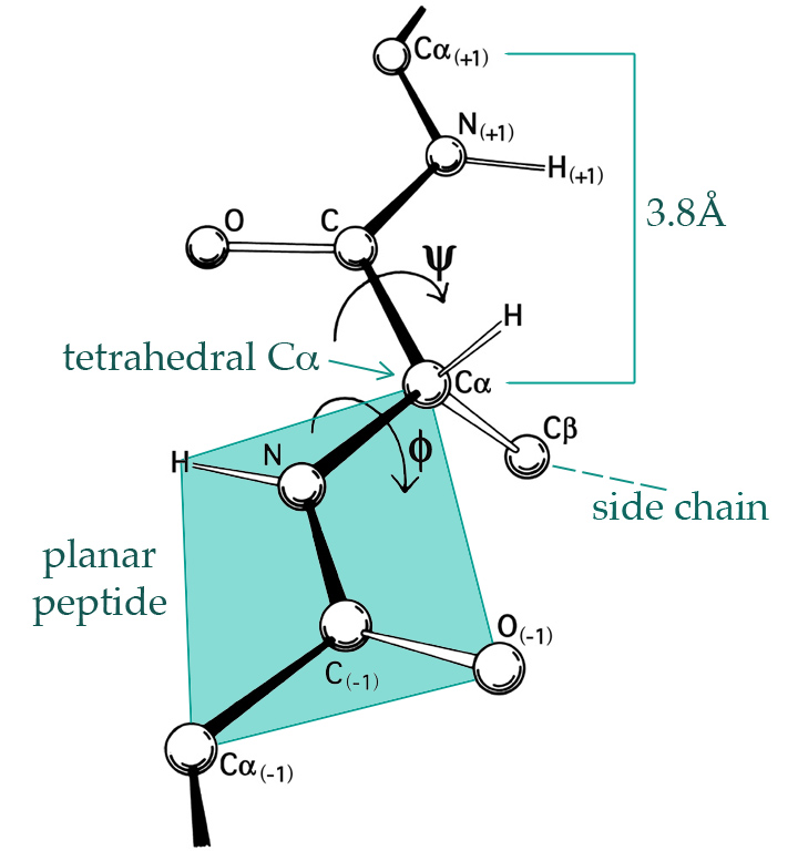
Figure 1.1: The 3D structure of proteins is largely given by the \(\phi\)- and \(\psi\)-angles of the peptide planes. By Dcrjsr, CC BY 3.0 via Wikimedia Commons.

A protein is a large molecule consisting of a backbone with carbon and nitrogen atoms arranged sequentially:

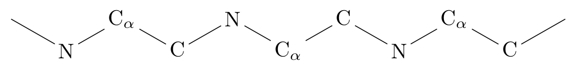
A hydrogen atom binds to each nitrogen (N) and an oxygen atom binds to each carbon without the \(\alpha\) subscript (C), see Figure 1.1, and such four atoms form together what is known as a peptide bond between two alpha-carbon atoms (C\(_{\alpha}\)). Each C\(_{\alpha}\) atom binds a hydrogen atom and an amino acid side chain. There are 20 naturally occurring amino acids in genetically encoded proteins, each having a three letter code (such as Gly for Glycine, Pro for Proline, etc.). The protein will typically form a complicated 3D structure determined by the amino acids, which in turn determine the \(\phi\)- and the \(\psi\)-angles between the peptide planes as shown on Figure 1.1.

We will consider a small data set, phipsi, of experimentally determined angles from a single protein, the human protein 1HMP, which is composed of two chains (denoted A and B). Figure 1.2 shows the 3D structure of the protein.

head(phipsi)

##   chain  AA pos     phi     psi
## 1     A Pro   5 -1.6219  0.2259
## 2     A Gly   6  1.1484 -2.8314
## 3     A Val   7 -1.4160  2.1191
## 4     A Val   8 -1.4927  2.3941
## 5     A Ile   9 -2.1815  1.4878
## 6     A Ser  10 -0.7525  2.5676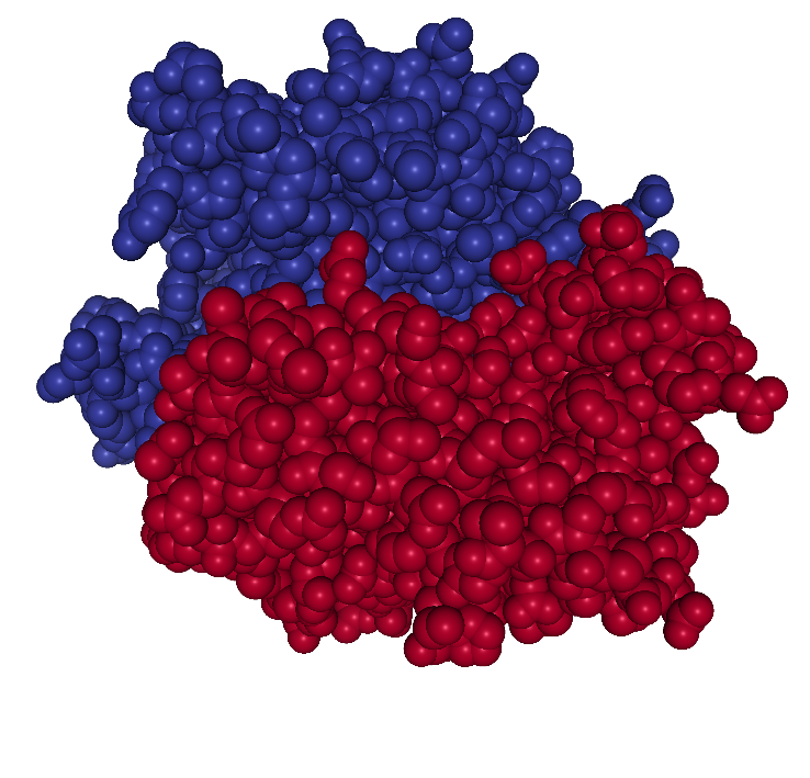

Figure 1.2: The 3D structure of the atoms constituting the protein 1HMP. The colors indicate the two different chains.

We can use base R functions such as hist() and density() to visualize the marginal distributions of the two angles.

hist(phipsi$phi, prob = TRUE)
rug(phipsi$phi)
density(phipsi$phi) %>% lines(col = "red", lwd = 2)

hist(phipsi$psi, prob = TRUE)
rug(phipsi$psi)
density(phipsi$psi) %>% lines(col = "red", lwd = 2)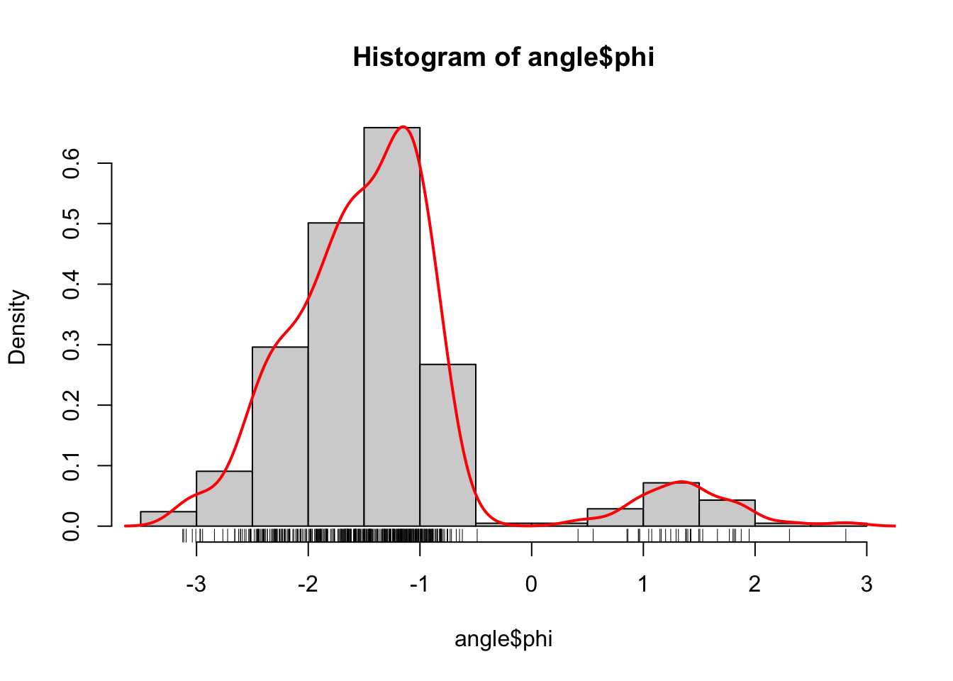

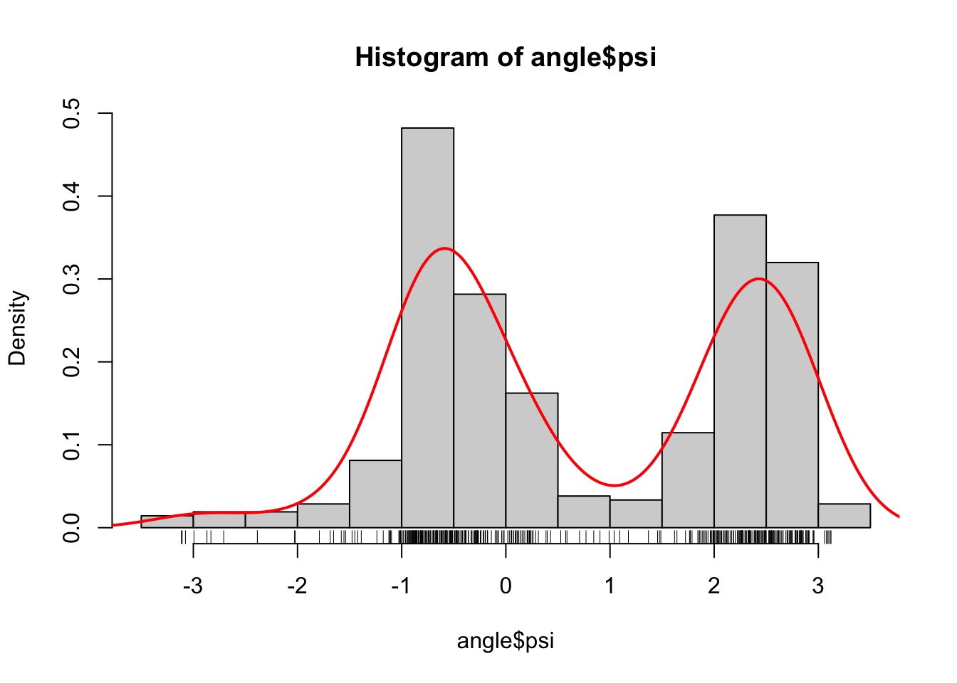
Figure 1.3: Histograms equipped with a rug plot and smoothed density estimate (red line) of the distribution of \(\phi\)-angles (left) and \(\psi\)-angles (right).

The smooth red density curve shown in Figure 1.3 can be thought of as a smooth version of a histogram. It is surprisingly difficult to find automatic smoothing procedures that perform uniformly well – it is even quite difficult to automatically select the number and positions of the breaks used for histograms. This is one of the important points that is taken up in this book: how to implement good default choices of various tuning parameters that are required by any smoothing procedure.

1.1.2 Using ggplot2

It is also possible to use ggplot2 to achieve similar results.

library(ggplot2)
ggplot(phipsi, aes(x = phi)) + 
  geom_histogram(aes(y = ..density..), bins = 13) + 
  geom_density(col = "red", linewidth = 1) + 
  geom_rug()

ggplot(phipsi, aes(x = psi)) + 
  geom_histogram(aes(y = ..density..), bins = 13) + 
  geom_density(col = "red", linewidth = 1) + 
  geom_rug()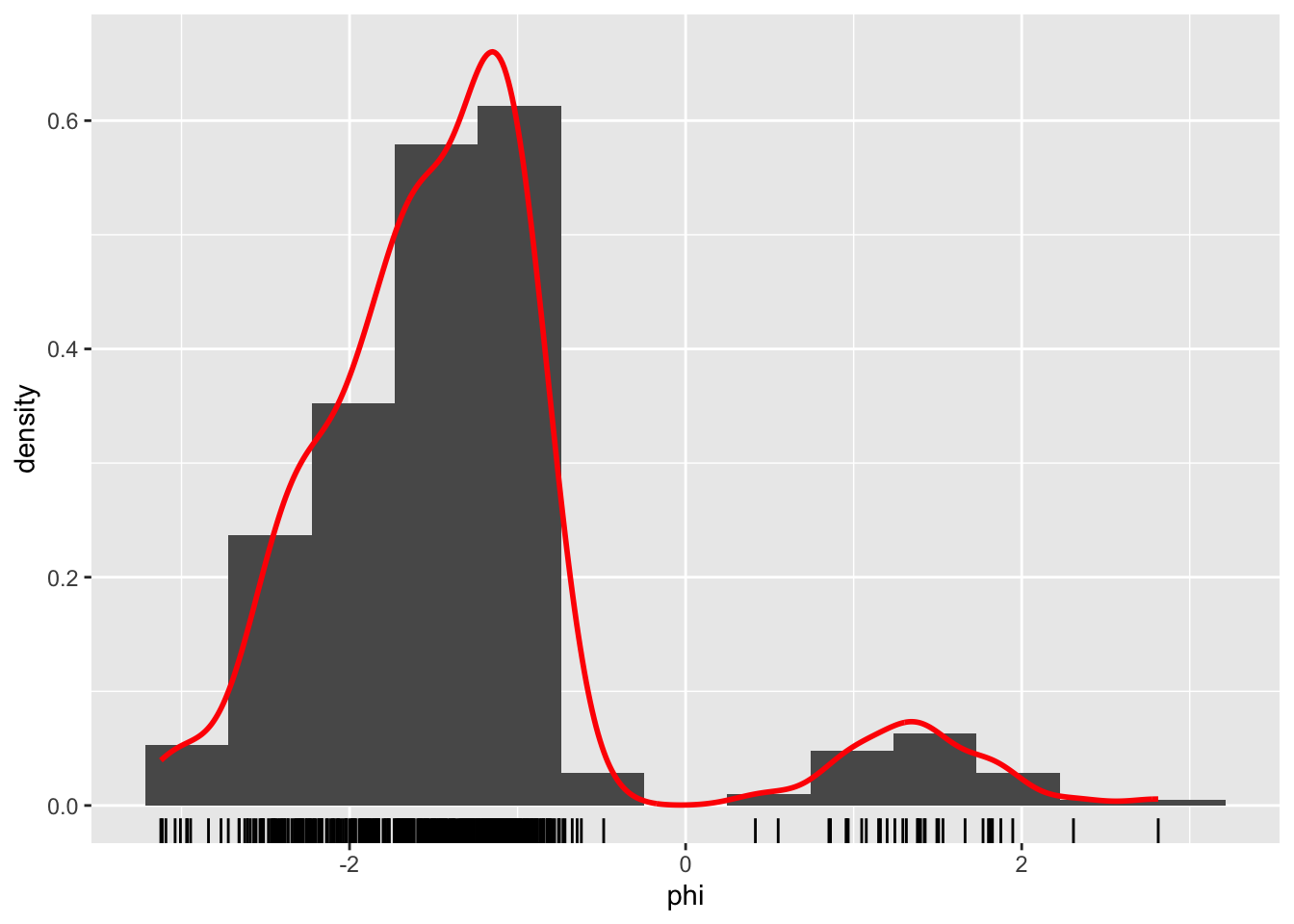

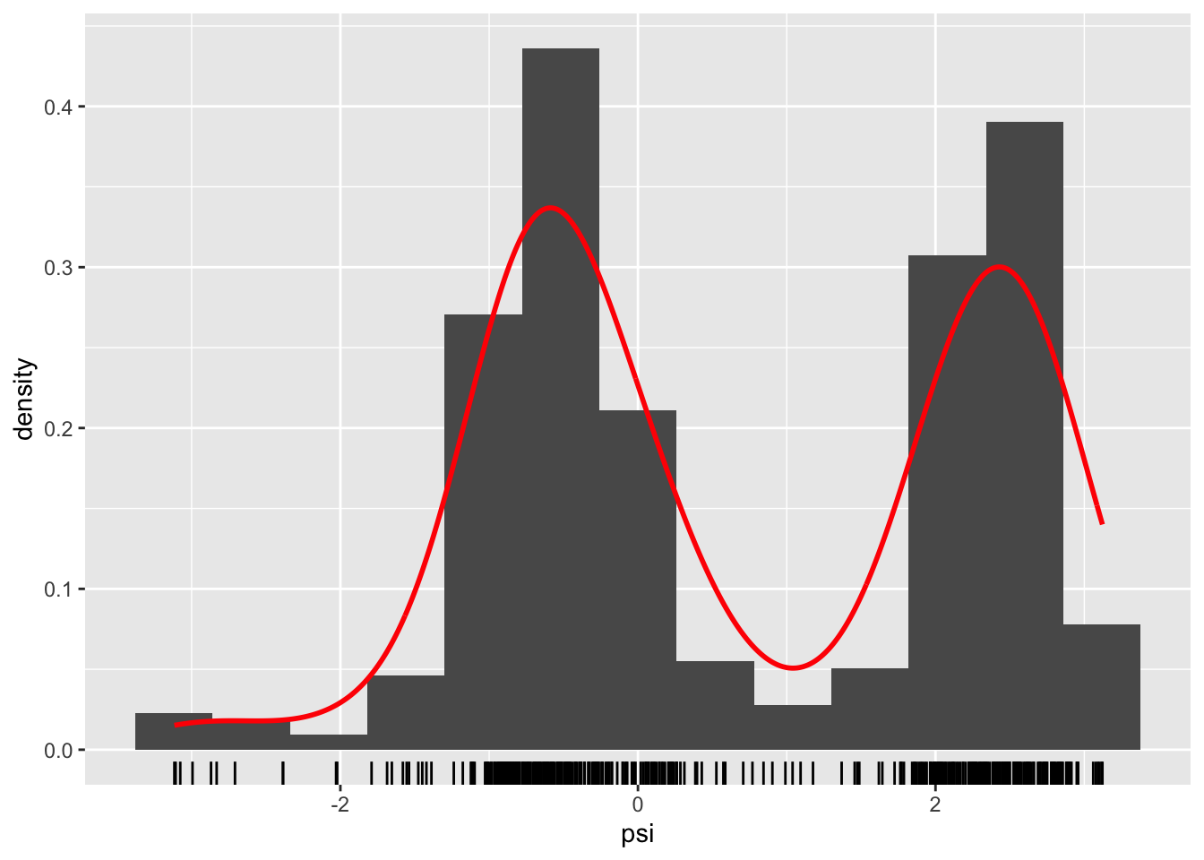
Figure 1.4: Histograms and density estimates of \(\phi\)-angles (left) and \(\psi\)-angles (right) made with ggplot2.

Histograms produced by ggplot2 have a non adaptive default number of bins equal to 30 (number of breaks equal to 31), which is different from hist that uses Sturges’ formula \[ \text{number of breaks} = \lceil \log_2(n) + 1 \rceil \] with \(n\) the number of observations in the data set. In addition, this number is further modified by the function pretty() that generates “nice” breaks, which results in 14 breaks for the angle data. For easier comparison, the number of bins used by geom_histogram() above is set to 13, though it should be noticed that the breaks are not chosen in exactly the same way by geom_histogram() and hist(). Automatic and data adaptive bin selection is difficult, and geom_histogram() implements a simple and fixed, but likely suboptimal, default while notifying the user that this default choice can be improved by setting binwidth.

For the density, geom_density() actually relies on the density() function and its default choices of how and how much to smooth. Thus the figure may have a slightly different appearance, but the estimated density obtained by geom_density() is identical to the one obtained by density().

1.1.3 Changing the defaults

The range of the angle data is known to be \((-\pi, \pi]\), which neither the histogram nor the density smoother take advantage of. The pretty() function, used by hist() chooses, for instance, breaks in \(-3\) and \(3\), which results in the two extreme bars in the histogram to be misleading. Note also that for the \(\psi\)-angle it appears that the defaults result in oversmoothing of the density estimate. That is, the density is more smoothed out than the data (and the histogram) appears to support.

To obtain different—and perhaps better—results, we can try to change some of the defaults of the histogram and density functions. The two most important defaults to consider are the bandwidth and the kernel. Postponing the mathematics to Chapter 2, the kernel controls how neighboring data points are weighted relatively to each other, and the bandwidth controls the size of neighborhoods. A bandwidth can be specified manually as a specific numerical value, but for a fully automatic procedure, it is selected by a bandwidth selection algorithm. The density() default is a rather simplistic algorithm known as Silverman’s rule-of-thumb.

hist(phipsi$psi, breaks = seq(-pi, pi, length.out = 15), prob = TRUE)
rug(phipsi$psi)
density(phipsi$psi, adjust = 1, cut = 0) %>% lines(col = "red", lwd = 2)
density(phipsi$psi, adjust = 0.5, cut = 0) %>% lines(col = "blue", lwd = 2)
density(phipsi$psi, adjust = 2, cut = 0) %>% lines(col = "purple", lwd = 2)

hist(phipsi$psi, breaks = seq(-pi, pi, length.out = 15), prob = TRUE)
rug(phipsi$psi)
# Default kernel is "gaussian"
density(phipsi$psi, bw = "SJ", cut = 0) %>% lines(col = "red", lwd = 2)
density(phipsi$psi, kernel = "epanechnikov", bw = "SJ", cut = 0) %>% 
  lines(col = "blue", lwd = 2)
density(phipsi$psi, kernel = "rectangular", bw = "SJ", cut = 0) %>% 
  lines(col = "purple", lwd = 2)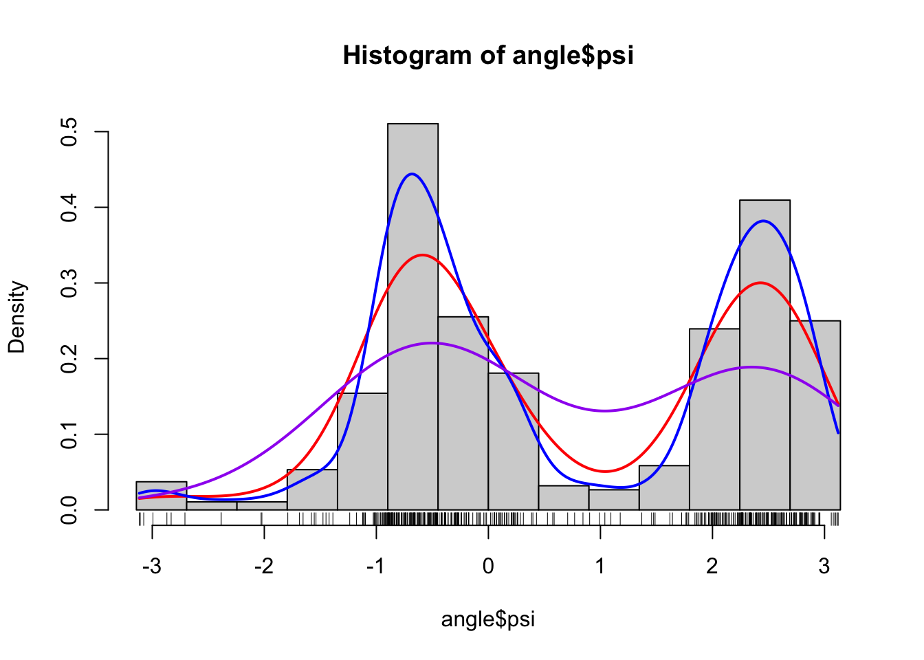

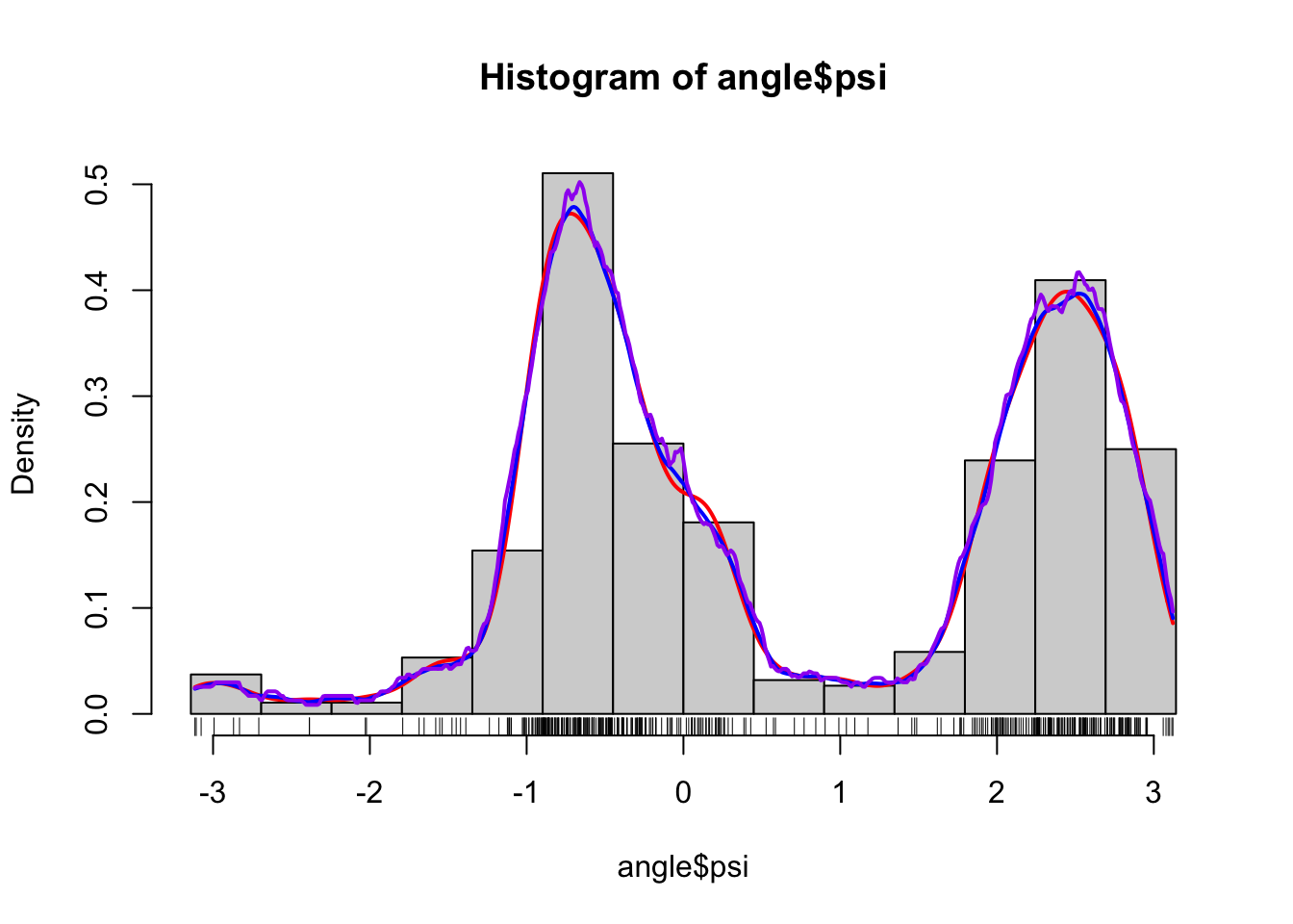
Figure 1.5: Histograms and various density estimates for the \(\psi\)-angles. The colors indicate different choices of bandwidth adjustments using the otherwise default bandwidth selection (left) and different choices of kernels using Sheather-Jones bandwidth selection (right).

Figure 1.5 shows examples of several different density estimates that can be obtained by changing the defaults of density. The breaks for the histogram have also been chosen manually to make sure that they match the range of the data. Note, in particular, that Sheather-Jones bandwidth selection appears to work better than the default bandwidth for this example. This is generally the case for multimodal distributions, where the default bandwidth tends to oversmooth. Note also that the choice of bandwidth is far more consequential than the choice of kernel, the latter mostly affecting how wiggly the density estimate is locally.

It should be noted that defaults arise as a combination of historically sensible choices and backward compatibility. Thought should go into choosing a good, robust default, but once a default is chosen, it should not be changed haphazardly, as this might break existing code. That is why not all defaults used in R are by today’s standards the best known choices. You see this argument made in the documentation of density regarding the default for bandwidth selection, where Sheather-Jones is suggested as a better default than the current, but for compatibility reasons Silverman’s rule-of-thumb is the default and is likely to remain being so.

1.1.4 Multivariate methods

This section provides a single illustration of how to use the bivariate kernel smoother kde2d from the MASS package for bivariate density estimation of the \((\phi, \psi)\)-angle distribution. A scatter plot of \(\phi\) and \(\psi\) angles is known as a Ramachandran plot, and it provides a classical and important way of visualizing local structural constraints of proteins in structural biochemistry. The density estimate can be understood as an estimate of the distribution of \((\phi, \psi)\)-angles in naturally occuring proteins from the small sample of angles in our data set.

We compute the density estimate in a grid of size 100 by 100 using a bandwidth of 2 and using the kde2d function that uses a bivariate normal kernel.

denshat <- MASS::kde2d(phipsi$phi, phipsi$psi, h = 2, n = 100)

denshat <- data.frame(
  cbind(
    denshat$x, 
    rep(denshat$y, each = length(denshat$x)), 
    as.vector(denshat$z)
    )
)

colnames(denshat) <- c("phi", "psi", "dens")
p <- ggplot(denshat, aes(phi, psi)) +
  geom_tile(aes(fill = dens), alpha = 0.5) +
  geom_contour(aes(z = sqrt(dens))) + 
  geom_point(data = phipsi, aes(fill = NULL)) +
  scale_fill_gradient(low = "white", high = "darkblue", trans = "sqrt")

We then recompute the density estimate in the same grid of size using the smaller bandwidth of 0.5.

denshat <- MASS::kde2d(phipsi$phi, phipsi$psi, h = 0.5, n = 100)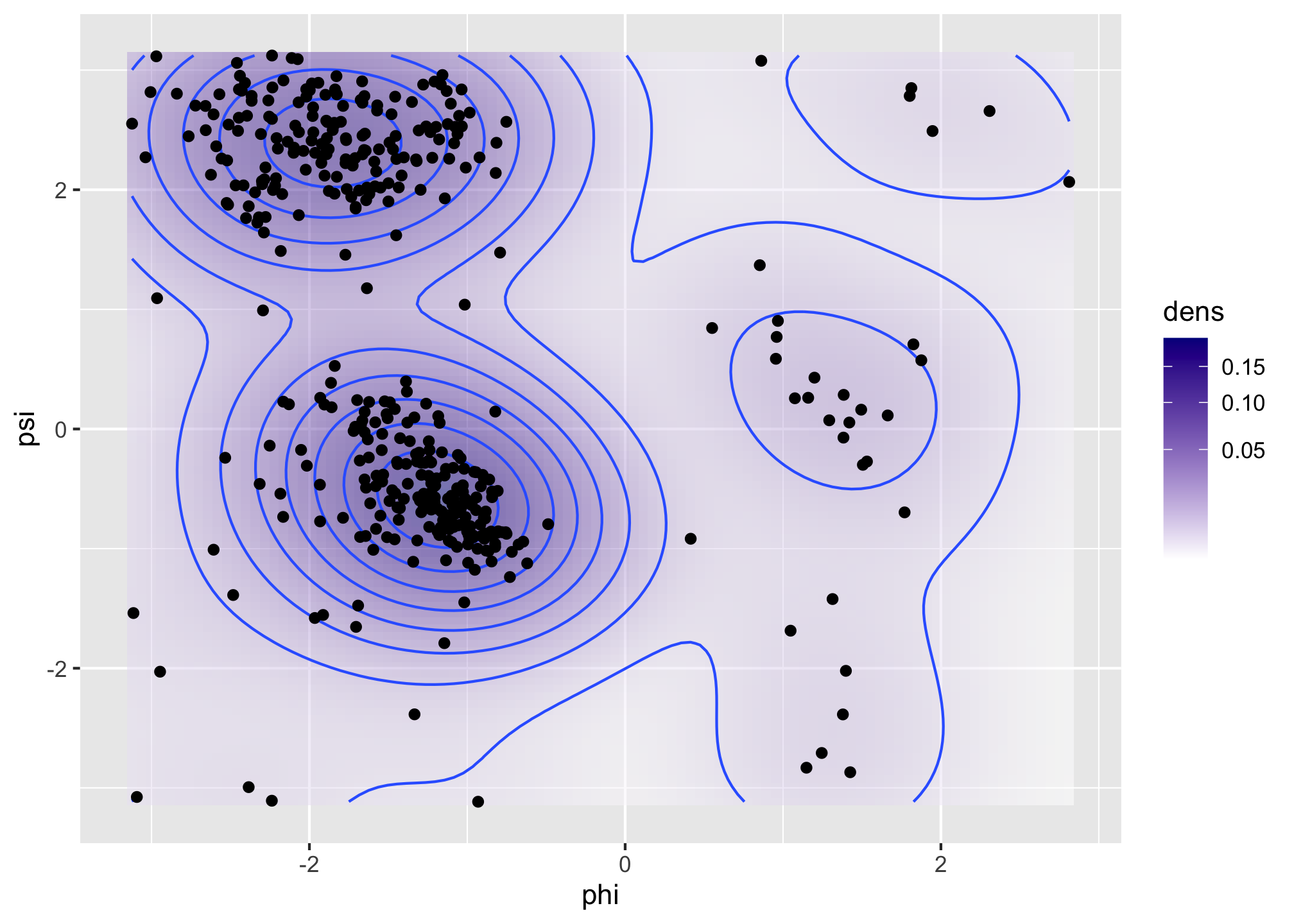

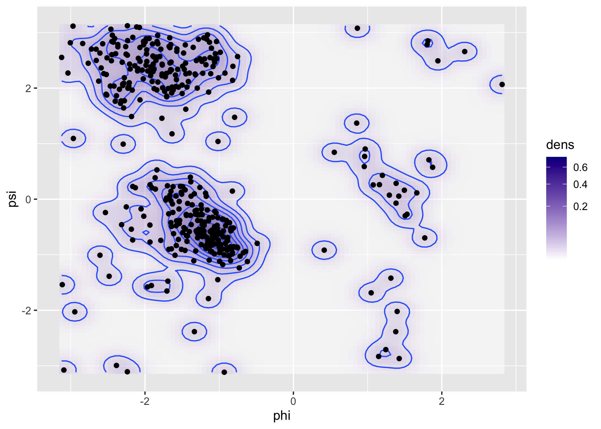
Figure 1.6: Bivariate density estimates of protein backbone angles using a bivariate Gaussian kernel with bandwiths \(2\) (left) and \(0.5\) (right).

The Ramachandran plot in Figure 1.6 shows how structural constraints of a protein, such as steric effects, induce a non-standard bivariate distribution of \((\phi, \psi)\)-angles.

1.1.5 Large scale smoothing

With small data sets of less than 10,000 data points, say, univariate smooth density estimation requires a very modest amount of computation. That is true even with rather naive implementations of the standard methods. The R function density is implemented using a number of computational tricks like binning and the fast Fourier transform, and it can compute density estimates with a million data points (around 8 MB) within a fraction of a second.

It is unclear if we ever need truly large scale univariate density estimation with terabytes of data points, say. If we have that amount of (heterogeneous) data it is likely that we are better off breaking the data down into smaller and more homogeneous groups. That is, we should turn a big data computation into a large number of small data computations. That does not remove the computational challenge but it does diminish it somewhat e.g. by parallelization.

Deng and Wickham did a review in 2011 on Density estimation in R, where they assessed the performance of a number of R packages including the density function. The KernSmooth package was singled out in terms of speed as well as accuracy for computing smooth density estimates with density performing quite well too. (Histograms are non-smooth density estimates and generally faster to compute). The assessment was based on using defaults for the different packages, which is meaningful in the sense of representing the performance that the occasional user will experience. It is, however, also an evaluation of the combination of default choices and the implementation, and as different packages rely on e.g. different bandwidth selection algorithms, this assessment is not the complete story. The bkde function from the KernSmooth package, as well as density, are solid choices, but the point is that performance assessment is a multifaceted problem.

To be a little more specific about the computational complexity of density estimators, suppose that we have \(n\) data points and want to evaluate the density in \(m\) points. A naive implementation of kernel smoothing, Section 2.2, has \(O(mn)\) time complexity, while a naive implementation of the best bandwidth selection algorithms have \(O(n^2)\) time complexity. As a simple rule-of-thumb, anything beyond \(O(n)\) will not scale to very large data sets. A quadratic time complexity for bandwidth selection will, in particular, be a serious bottleneck. Kernel smoothing illustrates perfectly that a literal implementation of the mathematics behind a statistical method may not always be computationally viable. Even the \(O(mn)\) time complexity may be quite a bottleneck as it reflects \(mn\) kernel evaluations, each being potentially a computationally relatively expensive operation.

The binning trick, with the number of bins set to \(m\), is a grouping of the data points into \(m\) sets of neighbor points (bins) with each bin representing the points in the bin via a single point and a weight. If \(m \ll n\), this can reduce the time complexity substantially to \(O(m^2) + O(n)\). The fast Fourier transform may reduce the \(O(m^2)\) term even further to \(O(m\log(m))\). Some approximations are involved, and it is of importance to evaluate the tradeoff between time and memory complexity on one side and accuracy on the other side.

Multivariate smoothing is a different story. While it is possible to generalize the basic ideas of univariate density estimation to arbitrary dimensions, the curse-of-dimensionality hits unconstrained smoothing hard – statistically as well as computationally. Multivariate smoothing is therefore still an active research area developing computationally tractable and novel ways of fitting smooth densities or conditional densities to multivariate or even high-dimensional data. A key technique is to make structural assumptions to alleviate the challenge of a large dimension, but there are many different assumptions possible, which makes the body of methods and theory richer and the practical choices much more difficult.

1.2 Monte Carlo methods

Broadly speaking, Monte Carlo methods are computations that rely on some form of random input in order to carry out a computation. The actual random input will be generated by a (pseudo)random number generator according to some distributional specifications, and the precise value of the computation will depend on the precise value of the random input but in a way where we understand the magnitude of the dependence quite well. In most cases we can make the dependence diminish by increasing the amount of random input.

In statistics it is quite interesting in itself that we can make the computer simulate data so that we can draw an example data set from a statistical model. However, the real usage of such simulations is almost always as a part of a Monte Carlo computation, where we repeat the simulation of data sets a large number of times and compute distributional properties of various statistics. This is just one of the most obvious applications of Monte Carlo methods in statistics and there are many others. Disregarding the specific computation of interest in applications, a core problem of Monte Carlo methods is efficient simulation of random variables from a given target distribution.

1.2.1 Univariate von Mises distributions

We will exemplify Monte Carlo computations by considering angle distributions just as in Section 1.1. The angles take values in the interval \((-\pi, \pi]\), and we will consider models based on the von Mises distribution on this interval, which has density

\[f(x) = \frac{1}{\varphi(\theta)} e^{\theta_1 \cos(x) + \theta_2 \sin(x)}\]

for \(\theta = (\theta_1, \theta_2)^T \in \mathbb{R}^2\). A common alternative parametrization is obtained by introducing \(\kappa = \|\theta\|_2 = \sqrt{\theta_1^2 + \theta_2^2}\), and (whenever \(\kappa \neq 0\)) \(\nu = \theta / \kappa = (\cos(\mu), \sin(\mu))^T\) for \(\mu \in (-\pi, \pi]\). Using the \((\kappa, \mu)\)-parametrization the density becomes
\[f(x) = \frac{1}{\varphi(\kappa \nu)} e^{\kappa \cos(x - \mu)}.\] The former parametrization in terms of \(\theta\) is, however, the canonical parametrization of the family of distributions as an exponential family, which is particularly useful for various likelihood estimation algorithms. The normalization constant

\[\begin{align*} \varphi(\kappa \nu) & = \int_{-\pi}^\pi e^{\kappa \cos(x - \mu)}\mathrm{d} x \\ & = 2 \pi \int_{0}^{1} e^{\kappa \cos(\pi x)}\mathrm{d} x = 2 \pi I_0(\kappa) \end{align*}\]

is given in terms of the modified Bessel function \(I_0\). We can easily compute and plot the density using R’s besselI implementation of the modified Bessel function.

phi <- function(k) 2 * pi * besselI(k, 0)
curve(exp(cos(x)) / phi(1), -pi, pi, lwd = 2, ylab = "density", ylim = c(0, 0.52))
curve(exp(2 * cos(x - 1)) / phi(2), col = "red", lwd = 2, add = TRUE)
curve(exp(0.5 * cos(x + 1.5)) / phi(0.5), col = "blue", lwd = 2, add = TRUE)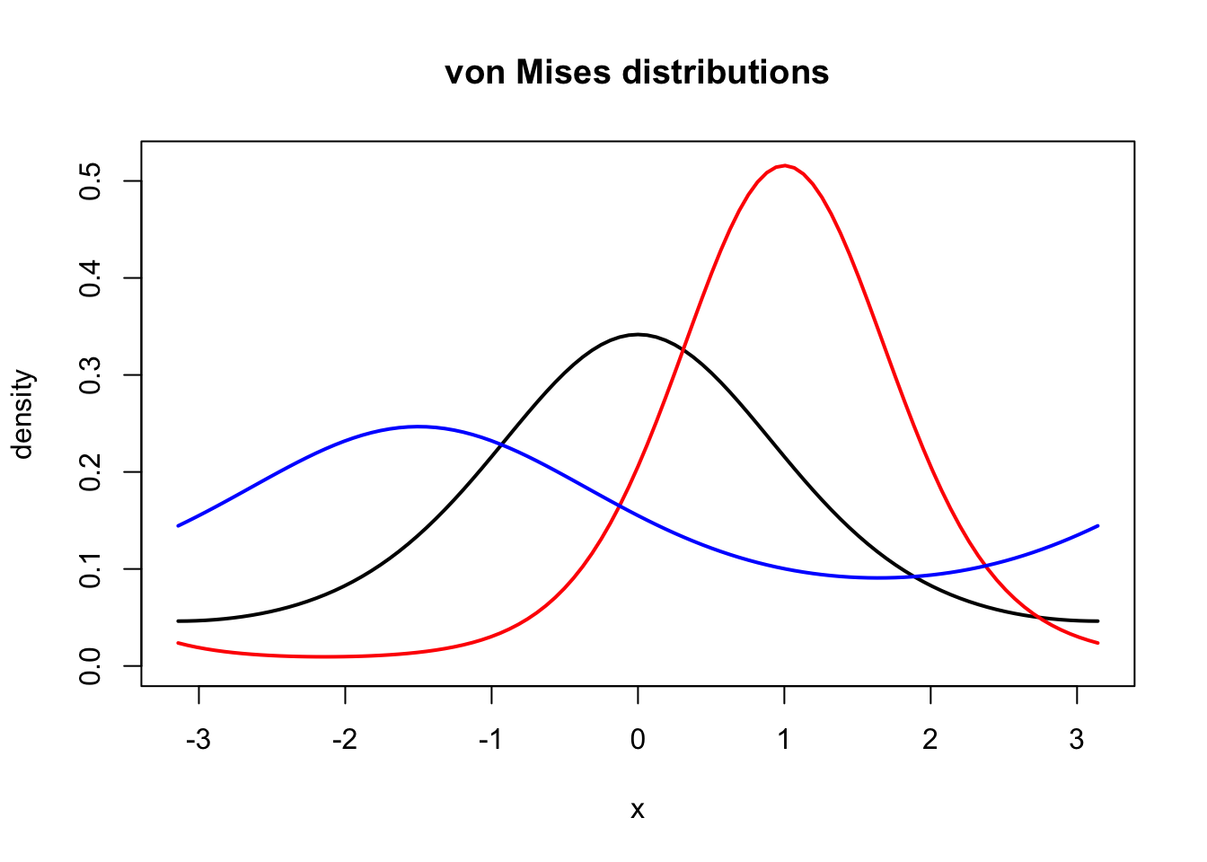

Figure 1.7: Density for the von Mises distribution with parameters \(\kappa = 1\) and \(\nu = 0\) (black), \(\kappa = 2\) and \(\nu = 1\) (red), and \(\kappa = 0.5\) and \(\nu = - 1.5\) (blue).

It is not entirely obvious how we should go about simulating data points from the von Mises distribution. It will be demonstrated in Section 4.3 how to implement a rejection sampler, which is one useful algorithm for simulating samples from a distribution with a density.

In this section we simply use the rmovMF function from the movMF package, which implements a few functions for working with (finite mixtures of) von Mises distributions, and even the general von Mises-Fisher distributions that are generalizations of the von Mises distribution to \(p\)-dimensional unit spheres.

library("movMF")
xy <- rmovMF(500, 0.5 * c(cos(-1.5), sin(-1.5)))
# rmovMF represents samples as elements on the unit circle
x <- acos(xy[, 1]) * sign(xy[, 2])

hist(x, breaks = seq(-pi, pi, length.out = 15), prob = TRUE)
rug(x)
density(x, bw = "SJ", cut = 0) %>% lines(col = "red", lwd = 2)
curve(exp(0.5 * cos(x + 1.5)) / phi(0.5), col = "blue", lwd = 2, add = TRUE)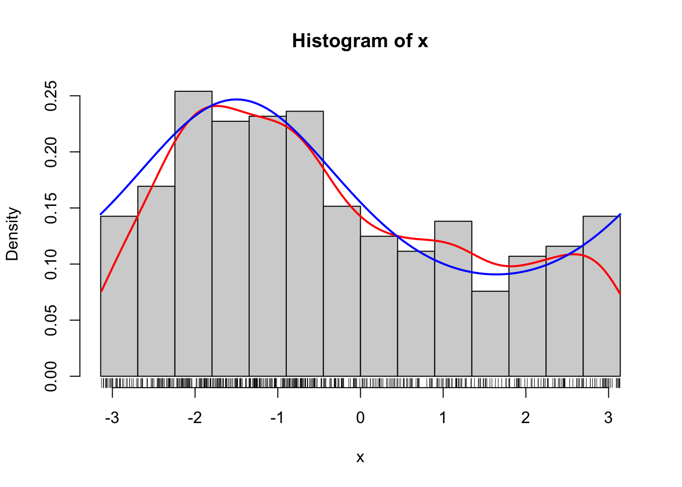

Figure 1.8: Histogram of 500 simulated data points from a von Mises distribution with parameters \(\kappa = 0.5\) and \(\nu = - 1.5\). A smoothed density estimate (red) and the true density (blue) are added to the plot.

1.2.2 Mixtures of von Mises distributions

The von Mises distributions are unimodal distributions on \((-\pi, \pi]\). Thus to find a good model of the bimodal angle data, say, we have do move beyond these distributions. A standard approach for constructing multimodal distributions is as mixtures of unimodal distributions. A mixture of two von Mises distributions can be constructed by flipping a (biased) coin to decide which of the two distributions to sample from. We will use the exponential family parametrization in the following.

thetaA <- c(3.5, -2)
thetaB <- c(-4.5, 4)
alpha <- 0.55 # Probability of von Mises distribution A
# The sample function implements the "coin flips"
u <- sample(c(1, 0), 500, replace = TRUE, prob = c(alpha, 1 - alpha))
xy <- rmovMF(500, thetaA) * u + rmovMF(500, thetaB) * (1 - u)
x <- acos(xy[, 1]) * sign(xy[, 2])

The rmovMF actually implements simulation from a mixture distribution directly, thus there is no need to construct the “coin flips” explicitly.

theta <- rbind(thetaA, thetaB)
xy <- rmovMF(length(x), theta, c(alpha, 1 - alpha))
x_alt <- acos(xy[, 1]) * sign(xy[, 2])

To compare the simulated data with two mixture components to the model and a smoothed density, we implement an R function that computes the density for an angle argument using the function dmovMF that takes a unit circle argument.

dvM <- function(x, theta, alpha) {
  xx <- cbind(cos(x), sin(x))
  dmovMF(xx, theta, c(alpha, 1 - alpha)) / (2 * pi)
}

Note that dmovMF uses normalized spherical measure on the unit circle as reference measure, thus the need for the \(2\pi\) division if we want the result to be comparable to histograms and density estimates that use Lebesgue measure on \((-\pi, \pi]\) as the reference measure.

hist(x, breaks = seq(-pi, pi, length.out = 15), prob = TRUE, ylim = c(0, 0.5))
rug(x)
density(x, bw = "SJ", cut = 0) %>% lines(col = "red", lwd = 2)
curve(dvM(x, theta, alpha), col = "blue", lwd = 2, add = TRUE)

hist(x_alt, breaks = seq(-pi, pi, length.out = 15), prob = TRUE, ylim = c(0, 0.5))
rug(x_alt)
density(x_alt, bw = "SJ", cut = 0) %>% lines(col = "red", lwd = 2)
curve(dvM(x, theta, alpha), col = "blue", lwd = 2, add = TRUE)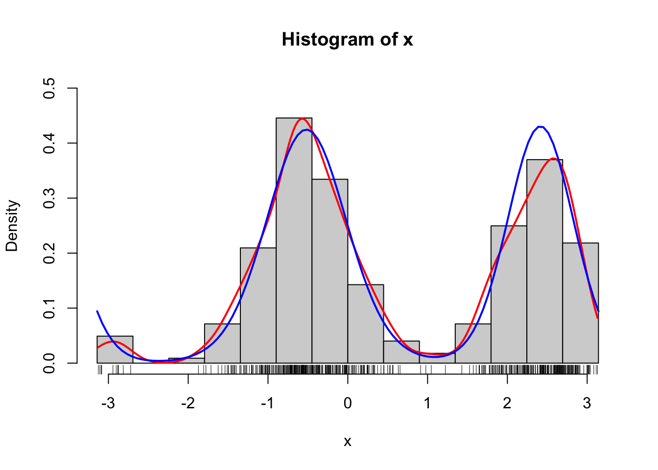

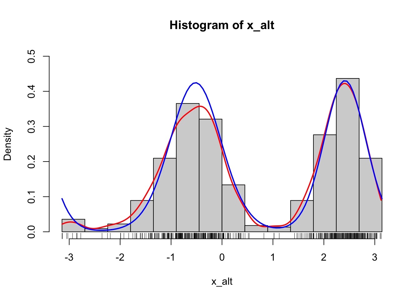
Figure 1.9: Histograms of 500 simulated data points from a mixture of two von Mises distributions using either the explicit construction of the mixture (left) or the functionality in rmovMF to simulate mixtures directly (right). A smoothed density estimate (red) and the true density (blue) are added to the plot.

Simulation of data from a distribution finds many applications. The technique is widely used whenever we want to investigate a statistical methodology in terms of its frequentistic performance under various data sampling models, and simulation is a tool of fundamental importance for the practical application of Bayesian statistical methods. Another important application is as a tool for computing approximations of integrals. This is usually called Monte Carlo integration and is a form of numerical integration. Computing probabilities or distribution functions, say, are notable examples of integrals, and we consider here the computation of the probability of the interval \((0, 1)\) for the above mixture of two von Mises distributions.

It is straightforward to compute this probability via Monte Carlo integration as a simple average. Note that we will use a large number of samples, 50,000 in this case, of simulated angles for this computation. Increasing the number even further will make the result more accurate. Chapter 5 deals with the assessment of the accuracy of Monte Carlo integrals, and how this random error can be estimated, bounded and minimized.

xy <- rmovMF(50000, theta, c(alpha, 1 - alpha))
x <- acos(xy[, 1]) * sign(xy[, 2])
mean(x > 0 & x < 1)  # Estimate of the probability of the interval (0, 1)

## [1] 0.08494

The probability above could, of course, be expressed using the distribution function of the mixture of von Mises distributions, which in turn can be computed in terms of integrals of von Mises densities. Specifically, the probability is \[p = \frac{\alpha}{\varphi(\theta_A)} \int_0^1 e^{\theta_{A, 1} \cos(x) + \theta_{A, 2} \sin(x)} \mathrm{d} x + \frac{1 - \alpha}{\varphi(\theta_B)} \int_0^1 e^{\theta_{B, 1} \cos(x) + \theta_{B, 2} \sin(x)} \mathrm{d} x,\] but these integrals do not have a simple analytic representation – just as the distribution function of the von Mises distribution doesn’t have a simple analytic expression. Thus the computation of the probability requires numerical computation of the integrals.

The R function integrate can be used for numerical integration of univariate functions using standard numerical integration techniques. We can thus compute the probability by integrating the density of the mixture, as implemented above as the R function dvM. Note the arguments passed to integrate below. The first argument is the density function, then follows the lower and the upper limits of the integration, and then follows additional arguments to the density – in this case parameter values.

integrate(dvM, 0, 1, theta = theta, alpha = alpha)

## 0.08635 with absolute error < 9.6e-16

The integrate function in R is an interface to a couple of classical QUADPACK Fortran routines for numerical integration via adaptive quadrature. Specifically, the computations rely on approximations of the form \[\int_a^b f(x) \mathrm{d} x \simeq \sum_i w_i f(x_i)\] for certain grid points \(x_i\) and weights \(w_i\), which are computed using Gauss-Kronrod quadrature. This method provides an estimate of the approximation error in addition to the numerical approximation of the integral itself.

It is noteworthy that integrate as a function implemented in R takes another function, in this case the density dvM, as an argument. R is a functional programming language and functions are first-class citizens. This implies, for instance, that functions can be passed as arguments to other functions using a variable name – just like any other variable can be passed as an argument to a function. In the parlance of functional programming, integrate is a functional: a higher-order function that takes a function as argument and returns a numerical value. One of the themes of this book is how to make good use of functional (and object oriented) programming features in R to write clear, expressive and modular code without sacrificing computational efficiency.

Returning to the specific problem of the computation of an integral, we may ask what the purpose of Monte Carlo integration is? Apparently we can just do numerical integration using e.g. integrate. There are at least two reasons why Monte Carlo integration is sometimes preferable. First, it is straightforward to implement and often works quite well for multivariate and even high-dimensional integrals, whereas grid-based numerical integration schemes scale poorly with the dimension. Second, it does not require that we have an analytic representation of the density. It is common in statistical applications that we are interested in the distribution of a statistic, which is a complicated transformation of data, and whose density is difficult or impossible to find analytically. Yet if we can just simulate data, we can simulate from the distribution of the statistic, and we can then use Monte Carlo integration to compute whatever probability or integral w.r.t. the distribution of the statistic that we are interested in.

1.2.3 Large scale Monte Carlo methods

Monte Carlo methods are used pervasively in statistics and in many other sciences today. It is nowadays trivial to simulate millions of data points from a simple univariate distribution like the von Mises distribution, and Monte Carlo methods are generally attractive because they allow us to solve computational problems approximately in many cases where exact or analytic computations are impossible and alternative deterministic numerical computations require more adaptation to the specific problem.

Monte Carlo methods are thus really good off-the-shelf methods, but scaling the methods up can be a challenge and is a contemporary research topic. For the simulation of multivariate \(p\)-dimensional data it can, for instance, make a big difference whether the algorithms scale linearly in \(p\) or like \(O(p^a)\) for some \(a > 1\). Likewise, some Monte Carlo methods (e.g.  Bayesian computations) depend on a data set of size \(n\), and for large scale data sets, algorithms that scale like \(O(n)\) are really the only algorithms that can be used in practice.

1.3 Optimization

The third part of the book is on optimization. This is a huge research field in itself and the focus of the book is on its relatively narrow application to parameter estimation in statistics. That is, when a statistical model is given by a parametrized family of probability distributions, optimization of some criterion, e.g., the likelihood function, is used to find a model that fits the data well.

Classical and generic optimization algorithms based on first and second order derivatives can often be used, but it is important to understand how convergence can be measured and monitored, and how the different algorithms scale with the size of the data set and the dimension of the parameter space. The choice of the right data structure, such as sparse matrices, can be pivotal for efficient implementations of the criterion function that is to be optimized.

For a mixture of von Mises distributions it is possible to compute the likelihood and optimize it using standard algorithms. However, it can also be optimized using the EM-algorithm, which is a clever algorithm for optimizing likelihood functions for models that can be formulated in terms of latent variables.

This section demonstrates how to fit a mixture of von Mises distributions to the angle data using the EM-algorithm as implemented in the R package movMF. This will illustrate some of the many practical choices we have to make when using numerical optimization such as: the choice of starting value; the stopping criterion; the precise specification of the steps that the algorithm should use; and even whether it should use randomized steps.

1.3.1 The EM-algorithm

The movMF() function implements the EM-algorithm for mixtures of von Mises distributions. The code below shows one example call of movMF() with one of the algorithmic control arguments specified. It is common in R that such arguments are all bundled together in a single list argument called control. It can make the function call appear a bit more complicated than it needed to be, but it allows for easier reuse of the – sometimes fairly long – list of control arguments. Note that as the movMF package works with data as elements on the unit circle, the angle data must be transformed using cos and sin.

psi_circle <- cbind(cos(phipsi$psi), sin(phipsi$psi))
vM_fit <- movMF(
  x = psi_circle, 
  k = 2,              # The number of mixture components
  control = list(
    start = "S"       # Determines how starting values are chosen
  )
)

The function movMF() returns an object of class movMF as the documentation says (see ?movMF). In this case it means that vM_fit is a list with a class label movMF, which controls how generic functions work for this particular list. When the object is printed, for instance, some of the the content of the list is formatted and printed as follows.

vM_fit

## theta:
##     [,1]   [,2]
## 1  3.473 -1.936
## 2 -4.508  3.873
## alpha:
## [1] 0.5487 0.4513
## L:
## [1] 193.3

What we see above is the estimated \(\theta\)-parameters for each of the two mixture components printed as a matrix, the mixture proportions (alpha) and the value of the log-likelihood function (L) in the estimated parameters.

We can compare the fitted model to the data using the density function as implemented above and the parameters estimated by the EM-algorithm.

hist(phipsi$psi, breaks = seq(-pi, pi, length.out = 15), prob = TRUE)
rug(phipsi$psi)
density(phipsi$psi, bw = "SJ", cut = 0) %>% lines(col = "red", lwd = 2)
curve(dvM(x, vM_fit$theta, vM_fit$alpha[1]), add = TRUE, col = "blue", lwd = 2)

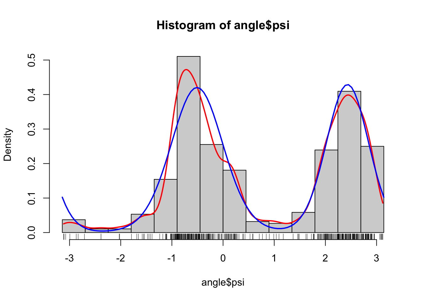
As we can see from the figure, this looks like a fairly good fit to the data, and this is reassuring for two reasons. First, it shows that the two-component mixture of von Mises distributions is a good model. This is a statistical reassurance. Second, it shows that the optimization over the parameter space found a good fit. This is a numerical reassurance. If we optimize over a parameter space and subsequently find that the model does not fit the data well, it is either because the numerical optimization failed or because the model is wrong.

Numerical optimization can fail for a number of reasons. For once, the algorithm can get stuck in a local optimum, but it can also stop prematurely either because the maximal number of iterations is reached or because the stopping criterion is fulfilled (even though the algorithm has not reached an optimum). Some information related to the two last problems can be gathered from the algorithm itself, and for movMF() such information is found in a list entry of vM_fit.

vM_fit$details

## $reltol
## [1] 1.49e-08
## 
## $iter
##    iter maxiter 
##      16     100 
## 
## $logLiks
## [1] 193.3
## 
## $E
## [1] "softmax"
## 
## $kappa
## NULL
## 
## $minalpha
## [1] 0
## 
## $converge
## [1] TRUE

We see that the number of iterations used was 16 (and less than the maximal number of 100), and the stopping criterion (small relative improvement) was active (converge is TRUE, if FALSE the algorithm is run for a fixed number of iterations). The tolerance parameter used for the stopping criterion was \(1.49 \times 10^{-8}\).

The small relative improvement criterion for stopping in iteration \(n\) is \[ |L(\theta_{n-1}) - L(\theta_n)| < \varepsilon (|L(\theta_{n-1})| + \varepsilon)\] where \(L\) is the log-likelihood and \(\varepsilon\) is the tolerance parameter above. The default tolerance parameter is the square root of the machine epsilon, see also ?.Machine. This is a commonly encountered default for a “small-but-not-too-small-number”, but outside of numerical differentiation this default may not be supported by much theory.

By choosing different control arguments we can change how the numerical optimization proceeds. A different method for setting the starting value is chosen below, which contains a random component. Here we consider the results in four different runs of the entire algorithm with different random starting values. We also decrease the number of maximal iterations to 10 and make the algorithm print out information about its progress along the way.

vM_control <- list(
    verbose = TRUE,   # Print output showing algorithmic progress
    maxiter = 10,     
    nruns = 4         # Effectively 4 runs with randomized starting values
  )
vM_fit <- movMF(psi_circle, 2, control = vM_control)
## Run: 1
## Iteration: 0 *** L: 158.572
## Iteration: 1 *** L: 190.999
## Iteration: 2 *** L: 193.118
## Iteration: 3 *** L: 193.238
## Iteration: 4 *** L: 193.279
## Iteration: 5 *** L: 193.293
## Iteration: 6 *** L: 193.299
## Iteration: 7 *** L: 193.3
## Iteration: 8 *** L: 193.301
## Iteration: 9 *** L: 193.301
## Run: 2
## Iteration: 0 *** L: 148.59
## Iteration: 1 *** L: 188.737
## Iteration: 2 *** L: 192.989
## Iteration: 3 *** L: 193.197
## Iteration: 4 *** L: 193.264
## Iteration: 5 *** L: 193.288
## Iteration: 6 *** L: 193.297
## Iteration: 7 *** L: 193.3
## Iteration: 8 *** L: 193.301
## Iteration: 9 *** L: 193.301
## Run: 3
## Iteration: 0 *** L: 168.643
## Iteration: 1 *** L: 189.946
## Iteration: 2 *** L: 192.272
## Iteration: 3 *** L: 192.914
## Iteration: 4 *** L: 193.157
## Iteration: 5 *** L: 193.249
## Iteration: 6 *** L: 193.282
## Iteration: 7 *** L: 193.295
## Iteration: 8 *** L: 193.299
## Iteration: 9 *** L: 193.301
## Run: 4
## Iteration: 0 *** L: 4.43876
## Iteration: 1 *** L: 5.33851
## Iteration: 2 *** L: 6.27046
## Iteration: 3 *** L: 8.54826
## Iteration: 4 *** L: 14.4429
## Iteration: 5 *** L: 29.0476
## Iteration: 6 *** L: 61.3225
## Iteration: 7 *** L: 116.819
## Iteration: 8 *** L: 172.812
## Iteration: 9 *** L: 190.518

In all four cases it appears that the algorithm is approaching the same value of the log-likelihood as what we found above, though the last run starts out in a much lower value and takes more iterations to reach a large log-likelihood value. Note also that in all runs the log-likelihood is increasing. It is a feature of the EM-algorithm that every step of the algorithm will increase the likelihood.

Variations of the EM-algorithm are possible, like in movMF where the control argument E determines the so-called E-step of the algorithm. Here the default (softmax) gives the actual EM-algorithm whereas hardmax and stochmax give alternatives. While the alternatives do not guarantee that the log-likelihood increases in every iteration they can be numerically beneficial. We rerun the algorithm from the same four starting values as above but using hardmax as the E-step. Note how we can reuse the control list by just adding a single element to it.

vM_control$E <- "hardmax"
vM_fit <- movMF(psi_circle, 2, control = vM_control)
## Run: 1
## Iteration: 0 *** L: 158.572
## Iteration: 1 *** L: 193.052
## Iteration: 2 *** L: 193.052
## Run: 2
## Iteration: 0 *** L: 148.59
## Iteration: 1 *** L: 192.443
## Iteration: 2 *** L: 192.812
## Iteration: 3 *** L: 193.052
## Iteration: 4 *** L: 193.052
## Run: 3
## Iteration: 0 *** L: 168.643
## Iteration: 1 *** L: 191.953
## Iteration: 2 *** L: 192.812
## Iteration: 3 *** L: 193.052
## Iteration: 4 *** L: 193.052
## Run: 4
## Iteration: 0 *** L: 4.43876
## Iteration: 1 *** L: 115.34
## Iteration: 2 *** L: 191.839
## Iteration: 3 *** L: 192.912
## Iteration: 4 *** L: 192.912

It is striking that all runs now stopped before the maximal number of iterations was reached, and run four is particularly noteworthy as it jumps from its low starting value to above 190 in just two iterations. However, hardmax is a heuristic algorithm, whose fixed points are not necessarily stationary points of the log-likelihood. We can also see above that all four runs stopped at values that are clearly smaller than the log-likelihood of about 193.30 that was reached using the real EM-algorithm. Whether this is a problem from a statistical viewpoint is a different matter; using hardmax could give an estimator that is just as efficient as the maximum likelihood estimator.

Which optimization algorithm should we then use? This is in general a very difficult question to answer, and it is non-trivial to correctly assess which algorithm is “the best”. As the application of movMF() above illustrates, optimization algorithms may have a number of different parameters that can be tweaked, and when it comes to actually implementing an optimization algorithm we need to: make it easy to tweak parameters; investigate and quantify the effect of the parameters on the algorithm; and choose sensible defaults. Without this work it is impossible to have a meaningful discussion about the benefits and deficits of various algorithms.

1.3.2 Large scale optimization

Numerical optimization is the tool that has made statistical models useful for real data analysis – most importantly by making it possible to compute maximum likelihood estimators in practice. This works very well when the model can be given a parametrization with a concave log-likelihood, while optimization of more complicated log-likelihood surfaces can be numerically challenging and lead to statistically dubious results.

In contemporary statistics and machine learning, numerical optimization has come to play an even more important role as structural model constraints are now often also part of the optimization, for instance via penalty terms in the criterion function. Instead of working with simple models selected for each specific problem and with few parameters, we use complex models with thousands or millions of parameters. They are flexible and adaptable but need careful, regularized optimization to not overfit the data. With large amounts of data the regularization can be turned down and we can discover aspects of data that the simple models would never show. However, we need to pay a computational price.

When the dimension of the parameter space, \(p\), and the number of data points, \(n\), are both large, evaluation of the log-likelihood or its gradient can become prohibitively costly. Optimization algorithms based on higher order derivatives are then completely out of the question, and even if the (penalized) log-likelihood and its gradient can be computed in \(O(pn)\)-operations this may still be too much for an optimization algorithm that does this in each iteration. Such large scale optimization problems have spurred a substantial development of stochastic gradient methods and related stochastic optimization algorithms that only use parts of data in each iteration, and which are currently the only way to fit sufficiently complicated models to data.