7 Monte Carlo integration
Suppose that we are interested in numerically computing the integral
\[ \int h_0(x) \mathrm{d} x \]
for some real valued function \(h_0\), how should we then proceed? A classical approach is to approximate the integral by a sum of the form
\[ \sum_{i=1}^N h_0(x_i) w_i. \]
Here the \(x_i\)-s are some, potentially carefully chosen, points in the \(x\)-space and \(w_i\) is the magnitude of the \(x\)-space where the values of \(h_0\) are well approximated by the value \(h_0(x_i)\). But how should we then in practice choose the \(x_i\)-s, and how should we compute the \(w_i\)-s?
If \(h_0(x) = h(x) f(x)\) for a probability density \(f\) we can get the idea of choosing the \(x_i\)-s randomly and simply take \(w_i = 1/N\). With \(X_1, \ldots, X_N\) i.i.d. with density \(f\) the Monte Carlo average satisfies that
\[ \hat{\mu}_{\textrm{MC}} := \frac{1}{N} \sum_{i=1}^N h(X_i) \rightarrow \mu := \E(h(X_1)) = \int h(x) f(x) \ \mathrm{d}x \]
for \(N \to \infty\) by the law of large numbers (LLN).
Monte Carlo integration is a clever idea, where we use the computer to simulate i.i.d. random variables and compute an average as an approximation of an integral. The idea may be applied in a statistical context, but it way also have applications outside of statistics and be a direct competitor to more standard numerical integration techniques. By increasing \(N\) the LLN tells us that the average will eventually become a good approximation of the integral. However, the LLN does not quantify how large \(N\) should be, and a fundamental question of Monte Carlo integration is therefore to quantify the precision of the average.
This chapter first deals with the quantification of the precision—mostly via the asymptotic variance in the central limit theorem. This will on the one hand provide us with a quantification of precision for any specific Monte Carlo approximation, and it will on the other hand provide us with a way to compare different Monte Carlo integration techniques.
The direct usage of the average above as an approximation of the integral requires that we can simulate directly from the distribution with density \(f\). This might be difficult or impossible, or it might just lead to Monte Carlo averages of very low precision. To remedy these challenges the subsequent sections treat importance sampling and variations thereof, which are techniques for simulating from a different distribution and use a weighted average to obtain the approximation of the integral.
7.1 Assessment
The error analysis of Monte Carlo integration differs from that of ordinary (deterministic) numerical integration methods. For the latter, error analysis provides bounds on the error of the computable approximation in terms of properties of the function to be integrated. Such bounds provide a guarantee on what the error at most can be. It is generally impossible to provide such a guarantee when using Monte Carlo integration because the computed approximation is by construction (pseudo)random. Thus the error analysis and assessment of the precision of \(\hat{\mu}_{\textrm{MC}}\) as an approximation of \(\mu\) will be probabilistic.
There are two main approaches. We can use approximations of the distribution of \(\hat{\mu}_{\textrm{MC}}\) to assess the precision by computing a confidence interval, say. Or we can provide finite sample upper bounds, known as concentration inequalities, on the probability that the error of \(\hat{\mu}_{\textrm{MC}}\) is larger than a given \(\varepsilon\). A concentration inequality can be turned into a confidence interval, if needed, or it can be used directly to answer a question such as: if I want the approximation to have an error smaller than \(\varepsilon = 10^{-3}\), how large does \(N\) need to be to guarantee this error bound with probability at least \(99.99\)%?
Confidence intervals are typically computed using the central limit theorem and an estimated value of the asymptotic variance. A major deficit of this method is that the central limit theorem does not provide bounds – only approximations whose precision for a finite \(N\) is often unclear. Thus without further analysis, we cannot really be certain that the results from the central limit theorem reflect the accuracy of \(\hat{\mu}_{\textrm{MC}}\).
Concentration inequalities provide actual guarantees, albeit probabilistic. They are, however, typically problem specific and harder to derive, they involve constants that are difficult to compute or bound, and they tend to be pessimistic in real applications.
An intermidiate approach is to use a simple and universal concentration inequality, such as Chebyshev’s inequality, and estimate the distribution specific constant (the variance) that enter into the bound it provides.
We will illustrate the use of both the central limit theorem and Chebyshev’s inequality for computing confidence intervals for Monte Carlo averages, but the focus in this chapter is on using the central limit theorem. We do, however, emphasize the example in Section 7.2.2 that shows how potentially misleading confidence intervals can be when the convergence is slow. The most notable practical challenge is estimation of the asymptotic variance, which can be quite poorly estimated for heavy tailed distributions.
7.1.1 Using the central limit theorem
The central limit theorem (CLT) gives that
\[ \hat{\mu}_{\textrm{MC}} = \frac{1}{N} \sum_{i=1}^N h(X_i) \overset{\textrm{approx}} \sim \mathcal{N}(\mu, \sigma^2_{\textrm{MC}} / n) \]
where
\[ \sigma^2_{\textrm{MC}} = V(h(X_1)) = \int (h(x) - \mu)^2 f(x) \ \mathrm{d}x. \]
We can estimate \(\sigma^2_{\textrm{MC}}\) using the empirical variance
\[ \hat{\sigma}^2_{\textrm{MC}} = \frac{1}{N - 1} \sum_{i=1}^N (h(X_i) - \hat{\mu}_{\textrm{MC}})^2, \]
then the variance of \(\hat{\mu}_{\textrm{MC}}\) is estimated as \(\hat{\sigma}^2_{\textrm{MC}} / N\) and a standard nominal 95% confidence interval for \(\mu\) is
\[ \hat{\mu}_{\textrm{MC}} \pm 1.96 \frac{\hat{\sigma}_{\textrm{MC}}}{\sqrt{N}}. \]
We illustrate the use of Monte Carlo integration and uncertainty quantification via the CLT by computing the mean of a Gamma distribution via Monte Carlo integration.
N <- 1000
x <- rgamma(N, 8) # h(x) = x
mu_hat <- (cumsum(x) / (1:N)) # Cumulative average
sigma_hat <- sd(x)
mu_hat[N]  # Theoretical value 8
## [1] 8.096
sigma_hat # Theoretical value sqrt(8) = 2.8284## [1] 2.862
ggplot(mapping = aes(1:N, mu_hat)) +
  geom_point() +
  geom_ribbon(
  mapping = aes(
    ymin = mu_hat - 1.96 * sigma_hat / sqrt(1:N),
    ymax = mu_hat + 1.96 * sigma_hat / sqrt(1:N)
  ), fill = "gray") +
  coord_cartesian(ylim = c(6, 10)) +
  geom_hline(yintercept = 8, color = "blue") +
  geom_line() +
geom_point() 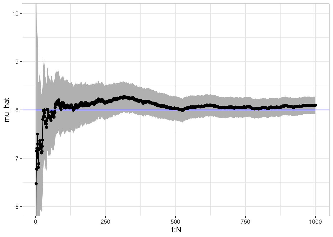
Figure 7.1: Sample path with pointwise 95% confidence band for Monte Carlo integration of the mean of a gamma distributed random variable.
Figure 7.1 shows the pointwise 95% confidence band for the Monte Carlo average. The CLT states in this particular case that
\[ \P\left( \hat{\mu}_{\textrm{MC}} - 1.96 \frac{\hat{\sigma}_{\textrm{MC}}}{\sqrt{N}} \leq 8 \leq \hat{\mu}_{\textrm{MC}} + 1.96 \frac{\hat{\sigma}_{\textrm{MC}}}{\sqrt{N}} \right) \to 0.95 \]
for \(N \to \infty\). This means that for \(N\) sufficiently large (but we do not know how large), the interval will cover the value \(\mu = 8\) of the integral with probability approximately 0.95. The actual coverage probability, that is, the probability on the left hand side above, may thus not be exactly 0.95, and for small \(N\) it can sometimes be much smaller.
7.1.2 Concentration inequalities
Since \(h(X_1)\) is a real valued random variable with finite second moment, \(\mu = \E(h(X_1))\) and \(\sigma^2 = \V(h(X_1))\), Chebychev’s inequality holds:
\[ \P(|h(X_1) - \mu| > \varepsilon) \leq \frac {\sigma^2}{\varepsilon^2} \]
for all \(\varepsilon > 0\). This inequality implies, for instance, that for the simple Monte Carlo average we have the inequality
\[ \P(|\hat{\mu}_{\textrm{MC}} - \mu| > \varepsilon) \leq \frac{\sigma^2_{\textrm{MC}}}{n\varepsilon^2}. \]
A common usage of this inequality is to actually prove the Law of Large Numbers: for any \(\varepsilon > 0\)
\[ \P(|\hat{\mu}_{\textrm{MC}} - \mu| > \varepsilon) \rightarrow 0 \]
for \(N \to \infty\). Or \(\hat{\mu}_{\textrm{MC}}\) converges in probability towards \(\mu\) as \(N\) tends to infinity.
The above convergence statement is a mathematical assurance that the Monte Carlo average \(\hat{\mu}_{\textrm{MC}}\) does, indeed, approximate \(\mu\) for \(N\) large. We can interpret this as a proof that Monte Carlo integration is, at least qualitatively, a sensible approach for numerical computation of an integral.
Chebychev’s inequality does, additionally, give a a quantitative statement about how accurate \(\hat{\mu}_{\textrm{MC}}\) is as an approximation of \(\mu\). Reorganizing the inequality above, we can write it as
\[ \P\left( \hat{\mu}_{\textrm{MC}} - \varepsilon \frac{\sigma_{\textrm{MC}}}{\sqrt{N}} \leq \mu \leq \hat{\mu}_{\textrm{MC}} + \varepsilon \frac{\sigma_{\textrm{MC}}}{\sqrt{N}} \right) > 1 - \frac{1}{\varepsilon^2} \]
Solving for \(1/\varepsilon^2 = 0.05\), say, gives \(\epsilon = \sqrt{1 / 0.05} = 4.47\), so if we knew \(\sigma_{\textrm{MC}}\) the confidence interval
\[ \hat{\mu}_{\textrm{MC}} \pm 4.47 \frac{\sigma_{\textrm{MC}}}{\sqrt{N}}. \]
would have guaranteed coverage larger than 95% for all \(N\). In practice, we would have to estimate \(\sigma_{\textrm{MC}}\), e.g., by the empirical standard deviation \(\hat{\sigma}_{\textrm{MC}}\), and we would effectively get the same confidence interval as obtained by the CLT, except that the \(0.975\) quantile \(1.96\) for the normal distribution is replaced by \(4.47\). This gives a wider interval—with some support from theory of having actual finite sample coverage being at least 95%. However, due to using the plug-in estimate \(\hat{\sigma}_{\textrm{MC}}\) of the standard deviation, we in fact loose any finite sample guarantees.
There are various strategies to obtain other concentration inequalities, that do not contain unknown and distribution dependent constants, which can give actual finite sample guarantees of coverage. These are beyond the scope of this book and we will use confidence intervals based on the CLT throughout. They are easy to use and practically useful, but just remember that they do not come with guarantees—and for heavy tailed distributions they can be misleading.
7.2 Importance sampling
When we are only interested in Monte Carlo integration, we do, in fact, not need to sample from the target distribution. We can sample from another distribution and use reweighting to compute the integral of interest.
We first observe that \[\begin{align} \mu = \int h(x) f(x) \ \mathrm{d}x & = \int h(x) \frac{f(x)}{g(x)} g(x) \ \mathrm{d}x \\ & = \int h(x) w^*(x) g(x) \ \mathrm{d}x \end{align}\]
whenever \(g\) is a density fulfilling that \[ g(x) = 0 \Rightarrow f(x) = 0. \]
With \(X_1, \ldots, X_N\) i.i.d. with density \(g\) we define the weights \[ w^*(X_i) = f(X_i) / g(X_i). \] The importance sampling estimator is then \[ \hat{\mu}_{\textrm{IS}}^* := \frac{1}{N} \sum_{i=1}^N h(X_i)w^*(X_i). \] It has mean \(\mu\), and it follows again by the LLN that \[ \hat{\mu}_{\textrm{IS}}^* \rightarrow \E(h(X_1) w^*(X_1)) = \mu. \]
We will illustrate the use of importance sampling by computing the mean in the gamma distribution via simulations from a Gaussian distribution, cf. also Section 7.1.1.
x <- rnorm(N, 10, 3)
w_star <- dgamma(x, 8) / dnorm(x, 10, 3)
mu_hat_IS <- (cumsum(x * w_star) / (1:N))
mu_hat_IS[N]  # Theoretical value 8
## [1] 7.995To assess the precision of the importance sampling estimate via the CLT we need the variance of the average just as for plain Monte Carlo integration. By the CLT
\[ \hat{\mu}_{\textrm{IS}}^* \overset{\textrm{approx}} \sim \mathcal{N}(\mu, \sigma^{*2}_{\textrm{IS}} / n) \]
where
\[ \sigma^{*2}_{\textrm{IS}} = V (h(X_1)w^*(X_1)) = \int (h(x) w^*(x) - \mu)^2 g(x) \ \mathrm{d}x. \]
The importance sampling variance can be estimated similarly as the Monte Carlo variance
\[ \hat{\sigma}^{*2}_{\textrm{IS}} = \frac{1}{N - 1} \sum_{i=1}^N (h(X_i)w^*(X_i) - \hat{\mu}_{\textrm{IS}}^*)^2, \]
and a 95% standard confidence interval is computed as
\[ \hat{\mu}^*_{\textrm{IS}} \pm 1.96 \frac{\hat{\sigma}^*_{\textrm{IS}}}{\sqrt{N}}. \]
sigma_hat_IS <- sd(x * w_star)
sigma_hat_IS  # Theoretical value ??
## [1] 3.5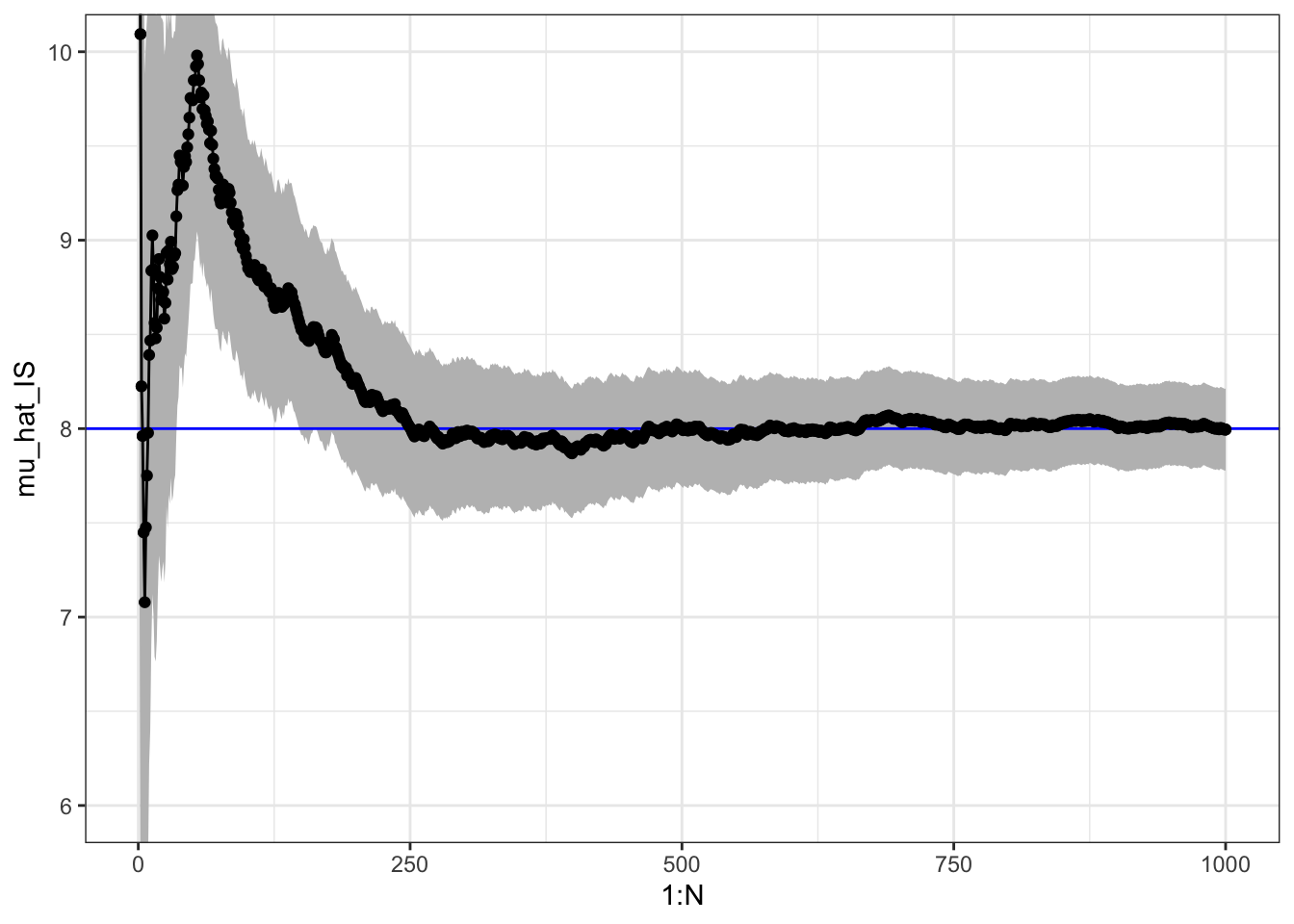
Figure 7.2: Sample path with confidence band for importance sampling Monte Carlo integration of the mean of a gamma distributed random variable via simulations from a Gaussian distribution.
It may happen that \(\sigma^{*2}_{\textrm{IS}} > \sigma^2_{\textrm{MC}}\) or \(\sigma^{*2}_{\textrm{IS}} < \sigma^2_{\textrm{MC}}\) depending on \(h\) and \(g\), but by choosing \(g\) cleverly so that \(h(x) w^*(x)\) becomes as constant as possible, importance sampling can often reduce the variance compared to plain Monte Carlo integration.
For the mean of the gamma distribution above, \(\sigma^{*2}_{\textrm{IS}}\) is about 50% larger than \(\sigma^2_{\textrm{MC}}\), so we loose precision by using importance sampling this way when compared to plain Monte Carlo integration. In Section 7.3 we consider a different example where we achieve a considerable variance reduction by using importance sampling.
7.2.1 Standardized weights
A slight modification of the importance sampling estimator consists of standardizing the weights so that they take values in \([0, 1]\) and sum to \(1\). This can sometimes be beneficial in itself, but it also allows for the use of importance sampling when the target density is only known up to a normalization constant.
Suppose that the target density is \(f = c^{-1} q\) with \(c\) unknown. Then
\[ c = \int q(x) \ \mathrm{d}x = \int \frac{q(x)}{g(x)} g(x) \ d x, \]
and
\[ \mu = \frac{\int h(x) w^*(x) g(x) \ d x}{\int w^*(x) g(x) \ d x}, \]
where \(w^*(x) = q(x) / g(x).\)
If \(X_1, \ldots, X_N\) are then i.i.d. from the distribution with density \(g\), an importance sampling estimate of \(\mu\) can be computed as
\[ \hat{\mu}_{\textrm{IS}} = \frac{\sum_{i=1}^N h(X_i) w^*(X_i)}{\sum_{i=1}^N w^*(X_i)} = \sum_{i=1}^N h(X_i) w(X_i), \]
where \(w^*(X_i) = q(X_i) / g(X_i)\) and
\[ w(X_i) = \frac{w^*(X_i)}{\sum_{i=1}^N w^*(X_i)} \]
are the standardized weights. This works irrespectively of the value of the normalizing constant \(c\), and it actually works if also \(g\) is unnormalized.
Revisiting the mean of the gamma distribution, we can implement importance sampling via sampling from a Gaussian distribution but using weights computed without the normalization constants.
w_star <- numeric(N)
x_pos <- x[x > 0]
w_star[x > 0] <- exp((x_pos - 10)^2 / 18 - x_pos + 7 * log(x_pos))
mu_hat_IS <- cumsum(x * w_star) / cumsum(w_star)
mu_hat_IS[N]  # Theoretical value 8
## [1] 8.102The variance of the IS estimator with standardized weights is a little more complicated, because the estimator is a ratio of random variables. From the multivariate CLT
\[ \frac{1}{N} \sum_{i=1}^N \left(\begin{array}{c} h(X_i) w^*(X_i) \\ w^*(X_i) \end{array}\right) \overset{\textrm{approx}}{\sim} \mathcal{N}\left( c \left(\begin{array}{c} \mu \\ {1} \end{array}\right), \frac{1}{N} \left(\begin{array}{cc} \sigma^{*2}_{\textrm{IS}} & \gamma \\ \gamma & \sigma^2_{w^*} \end{array} \right)\right), \]
where
\[\begin{align} \sigma^{*2}_{\textrm{IS}} & = V(h(X_1)w^*(X_1)) \\ \gamma & = \mathrm{cov}(h(X_1)w^*(X_1), w^*(X_1)) \\ \sigma_{w^*}^2 & = V (w^*(X_1)). \end{align}\]
We can then apply the \(\Delta\)-method with \(t(x, y) = x / y\). Note that \(Dt(x, y) = (1 / y, - x / y^2)\), whence
\[ Dt(c\mu, c) \left(\begin{array}{cc} \hat{\sigma}^{*2}_{\textrm{IS}} & \gamma \\ \gamma & \sigma^2_{w^*} \end{array} \right) Dt(c\mu, c)^T = c^{-2} (\sigma^{*2}_{\textrm{IS}} + \mu^2 \sigma_{w^*}^2 - 2 \mu \gamma). \]
By the \(\Delta\)-method
\[ \hat{\mu}_{\textrm{IS}} \overset{\textrm{approx}}{\sim} \mathcal{N}(\mu, c^{-2} (\sigma^{*2}_{\textrm{IS}} + \mu^2 \sigma_{w^*}^2 - 2 \mu \gamma) / n). \]
The unknown quantities in the asymptotic variance must be estimated using e.g. their empirical equivalents, and if \(c \neq 1\) (we have used unnormalized densities) it is necessary to estimate \(c\) as \(\hat{c} = \frac{1}{N} \sum_{i=1}^N w^*(X_i)\) to compute an estimate of the variance.
For the example with the mean of the gamma distribution, we find the following estimate of the variance.
c_hat <- mean(w_star)
sigma_hat_IS <- sd(x * w_star)
sigma_hat_w_star <- sd(w_star)
gamma_hat <- cov(x * w_star, w_star)
sigma_hat_IS_w <- sqrt(sigma_hat_IS^2 + mu_hat_IS[N]^2 * sigma_hat_w_star^2 -
                         2 * mu_hat_IS[N] * gamma_hat) / c_hat
sigma_hat_IS_w
## [1] 3.198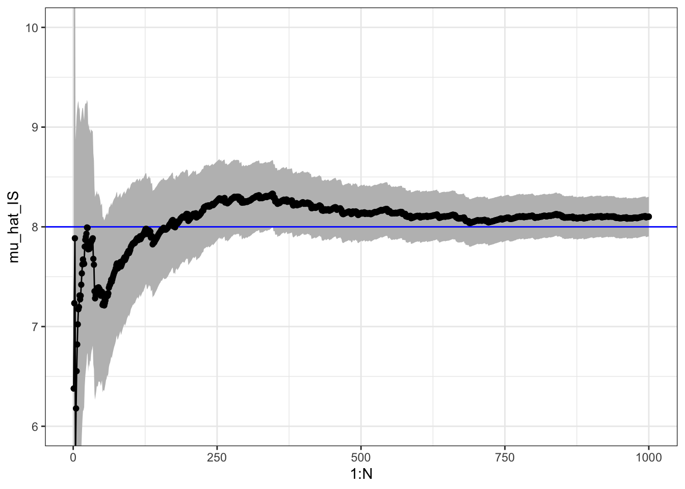
Figure 7.3: Sample path with confidence band for importance sampling Monte Carlo integration of the mean of a gamma distributed random variable via simulations from a Gaussian distribution and using standardized weights.
In this example, the variance when using standardized weights is a little lower than using unstandardized weights, but still larger than the variance for the plain Monte Carlo average.
7.2.2 Computing a high-dimensional integral
To further illustrate the usage, but also the limitations, of Monte Carlo integration and importance sampling, suppose we want to compute the \(p\)-dimensional integral
\[ \int h_0(x) \mathrm{d} x \]
w.r.t. Lebesgue measure in \(\mathbb{R}^p\) for some integrable function \(h_0\). We use the same idea as in importance sampling to rewrite the integral as an expectation w.r.t. a probability distribution. For simplicity, let us focus on sampling from a standard Gaussian distribution \(\mathcal{N}(0, I_p)\), with density \(g(x) = (2\pi)^{-p/2} \exp(-\|x\|_2^2/2)\). Then
\[\begin{align*} \int h_0(x) \mathrm{d} x & = \int h_0(x) \frac{g(x)}{g(x)} \mathrm{d} x \\ & = (2\pi)^{p/2} \int h(x) g(x) \mathrm{d} x \\ & = (2\pi)^{p/2} \E( h(X)), \end{align*}\]
where \(h(x) = h_0(x) \exp( \|x\|_2^2/2)\) and \(X \sim \mathcal{N}(0, I_p)\). Here we have incorporated the weights \(w^*(x) = \exp( \|x\|_2^2/2)\) into the function \(h\).
We now choose the specific function
\[ h_0(x) = \exp\left(-\frac{1}{2}\left(x_1^2 + \sum_{i=2}^p (x_k - \alpha x_{k-1})^2\right)\right). \]
Since \(x_1^2 + \sum_{i=2}^p (x_k - \alpha x_{k-1})^2 = \|x\|_2^2 + \sum_{i = 2}^p \alpha^2 x_{k-1}^2 - 2\alpha x_k x_{k-1}\), we have
\[ h(x) = \exp\left(- \frac{1}{2} \sum_{i = 2}^p \alpha^2 x_{k-1}^2 - 2\alpha x_k x_{k-1}\right). \]
Thus if \(X \sim \mathcal{N}(0, I_p)\), we have
\[ \int h_0(x) \mathrm{d} x = (2 \pi)^{p/2} \E\left( h(X) \right) = (2 \pi)^{p/2} \E\left( e^{- \frac{1}{2} \sum_{i = 2}^p \alpha^2 X_{k-1}^2 - 2\alpha X_k X_{k-1}} \right). \]
In the Monte Carlo integration below we ignore the factor \((2 \pi)^{p/2}\) and compute
\[ \mu = \E\left( \exp\left(- \frac{1}{2} \sum_{i = 2}^p \alpha^2 X_{k-1}^2 - 2\alpha X_k X_{k-1} \right) \right) \]
by generating \(p\)-dimensional random variables from \(\mathcal{N}(0, I_p)\). The value of the expectation can actually be computed analytically to be \(\mu = 1\), see Exercise 7.1.
First, we implement the function we want to integrate.
h <- function(x, alpha = 0.1){
  p <- length(x)
  tmp <- alpha * x[1:(p - 1)]
  exp( - sum((tmp / 2 - x[2:p]) * tmp))
}
Then we specify various parameters.
N <- 10000 # The number of random variables to generate
p <- 100   # The dimension of each random variable
The actual computation is implemented using the apply function. We
first look at the case with \(\alpha = 0.1\).
## [1] 0.9987We plot the cumulative average in Figure 7.4 and compare it to the actual value of the integral that we know is 1. We add pointwise 95% confidence intervals to plot—using either Chebychev’s inequality or the CLT.
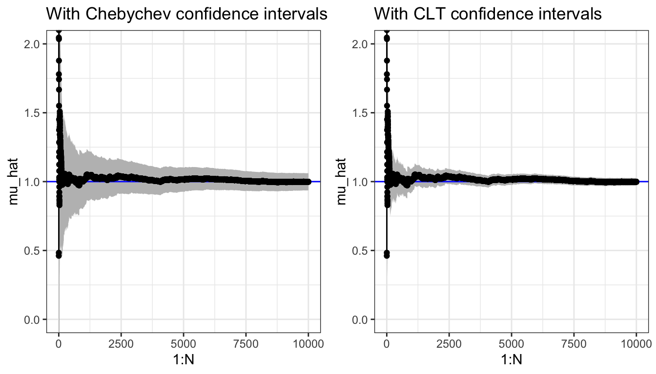
Figure 7.4: Sample path for the Monte Carlo average (\(\alpha = 0.1\))and pointwise 95% confidence intervals using either Chebychev’s inequality or the CLT.
The confidence bands provided by the CLT are typically more accurate estimates of the actual uncertainty than the upper bounds provided by Chebychev’s inequality.
To illustrate the limitations of Monte Carlo integration we increase \(\alpha\) to \(\alpha = 0.4\).
evaluations <- apply(x, 1, h, alpha = 0.4)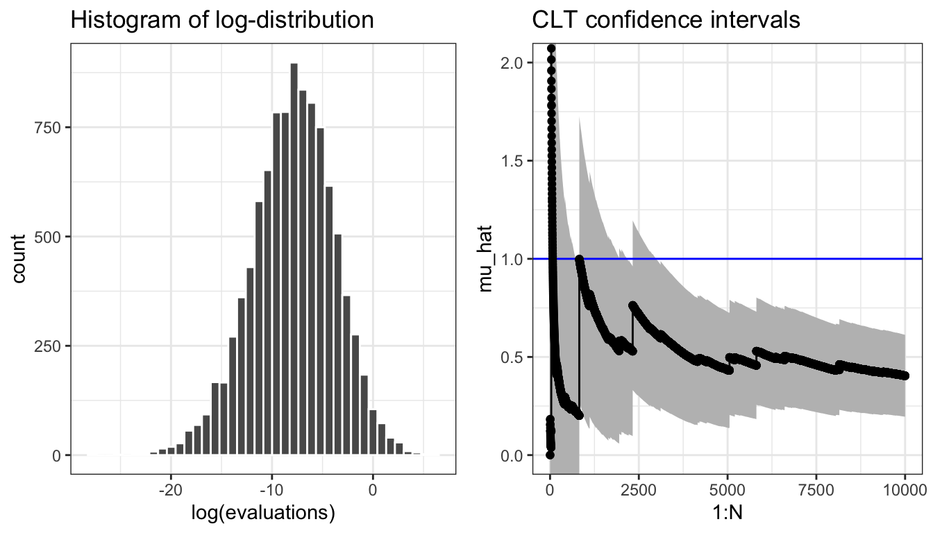
Figure 7.5: Histogram of the log-distribution and sample path for the Monte Carlo average (\(\alpha = 0.4\)) and pointwise 95% confidence intervals based on the CLT.
The sample path in Figure 7.5 is not carefully selected to be pathological. Due to occasional large values, the typical sample path will show occasional large jumps, and the variance may easily be grossly underestimated. The histogram of the log-distribution of the terms that enter into the Monte Carlo average also shows how there is several orders of magnitude differences between the typical values and the largest values. Figure 7.6 shows four additional sample paths where the confidence interval for \(N = 1000\) for three of them completely misses the actual value \(\mu = 1\), while the last is extremely wide. In this example the Monte Carlo integration technique does not perform well for \(\alpha = 0.4\) (or larger), and the uncertainty quantification via the CLT is highly unreliable.
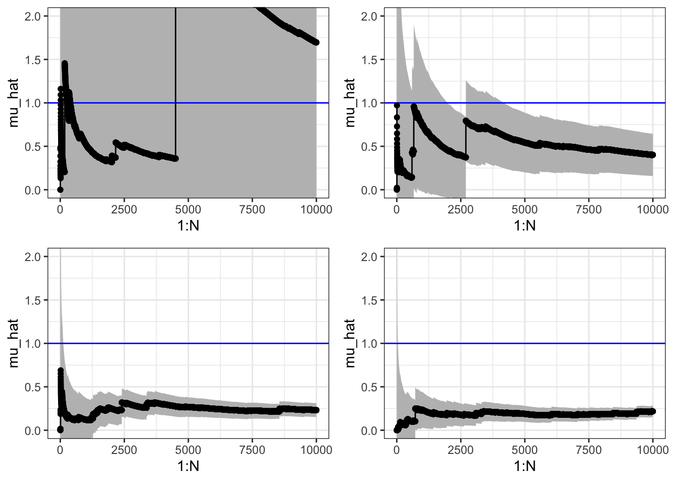
Figure 7.6: Four sample paths for the Monte Carlo average (\(\alpha = 0.4\)) and pointwise 95% confidence intervals based on the CLT.
To be fair, it is the choice of a standard multivariate normal distribution as the reference distribution for large \(\alpha\) that is problematic rather than Monte Carlo integration and importance sampling as such. However, in high dimensions it can be difficult to choose a suitable distribution to sample from.
The difficulty for the specific integral is due to the exponent of the integrand, which can become large and positive if \(x_k \approx x_{k-1}\) for enough coordinates. This happens rarely for independent random variables, but large values of rare events can, nevertheless, contribute notably to the integral. The larger \(\alpha \in (0, 1)\) is, the more pronounced is the problem with occasional large values of the integrand. It is possible to use importance sampling and instead sample from a distribution where the large values are more likely. For this particular example we would need to simulate from a distribution where the variables are dependent, and we will not pursue that here.
7.3 Network failure
In this section we consider a more serious application of importance sampling. Though still a toy example, where we can find an exact solution, the example illustrates well the type of application where we want to approximate a small probability using a Monte Carlo average. Importance sampling can then increase the probability of the rare event and as a result make the variance of the Monte Carlo average smaller.
We will consider the following network consisting of ten nodes and with some of the nodes connected.
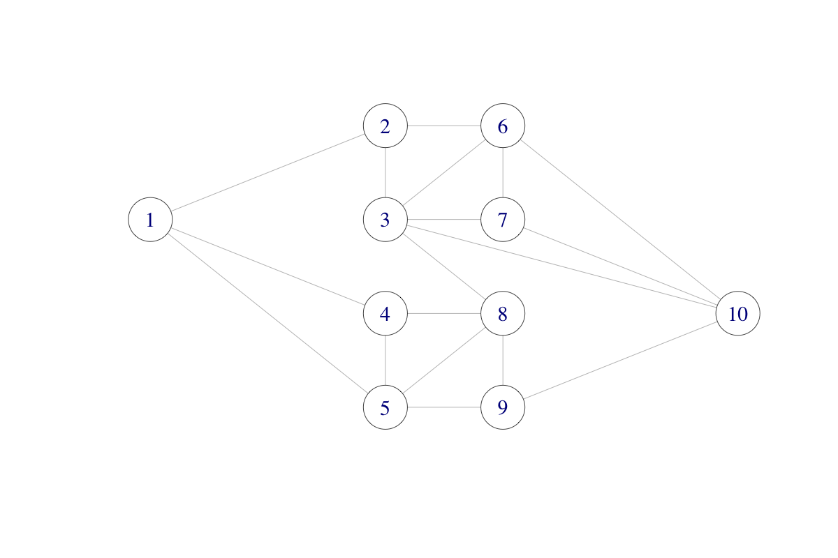
The network could be a computer network with ten computers. The different connections (edges) may “fail” independently with probability \(p\), and we ask the question: what is the probability that node 1 and node 10 are disconnected?
We can answer this question by computing an integral of an indicator function, that is, by computing the sum
\[ \mu = \sum_{x \in \{0,1\}^{18}} 1_B(x) f_p(x) \]
where \(f_p(x)\) is the point probability of \(x\), with \(x\) representing which of the 18 edges in the graph that fail, and \(B\) representing the set of edges where node 1 and node 10 are disconnected. By simulating edge failures we can approximate the sum as a Monte Carlo average.
The network of nodes can be represented as a graph adjacency matrix \(A\) such that \(A_{ij} = 1\) if and only if there is an edge between \(i\) and \(j\) (and \(A_{ij} = 0\) otherwise).
A # Graph adjacency matrix## [,1] [,2] [,3] [,4] [,5] [,6] [,7] [,8] [,9] [,10]
## [1,] 0 1 0 1 1 0 0 0 0 0
## [2,] 1 0 1 0 0 1 0 0 0 0
## [3,] 0 1 0 0 0 1 1 1 0 1
## [4,] 1 0 0 0 1 0 0 1 0 0
## [5,] 1 0 0 1 0 0 0 1 1 0
## [6,] 0 1 1 0 0 0 1 0 0 1
## [7,] 0 0 1 0 0 1 0 0 0 1
## [8,] 0 0 1 1 1 0 0 0 1 0
## [9,] 0 0 0 0 1 0 0 1 0 1
## [10,] 0 0 1 0 0 1 1 0 1 0To compute the probability that 1 and 10 are disconnected by Monte Carlo integration, we need to sample (sub)graphs by randomly removing some of the edges. This is implemented using the upper triangular part of the (symmetric) adjacency matrix.
sim_net <- function(Aup, p) {
  ones <- which(Aup == 1)
  Aup[ones] <- sample(
    c(0, 1),
    length(ones),
    replace = TRUE,
    prob = c(p, 1 - p)
  )
  Aup
}
The core of the implementation above uses the sample() function, which
can sample with replacement from the set \(\{0, 1\}\). The vector ones
contains indices of the (upper triangular part of the) adjacency matrix
containing a 1, and these positions are replaced by the sampled values before
the matrix is returned.
It is fairly fast to sample even a large number of random graphs this way.
Aup <- A
Aup[lower.tri(Aup)] <- 0
bench::bench_time(replicate(1e5, {sim_net(Aup, 0.5); NULL}))
## process real
## 675ms 665msThe second function we implement checks network connectivity based on the upper triangular part of the adjacency matrix. It relies on the fact that there is a path from node 1 to node 10 consisting of \(m\) edges if and only if \((A^m)_{1,10} > 0\). We see directly that such a path needs to consist of at least \(m = 3\) edges. Also, we do not need to check paths with more than \(m = 9\) edges as they will contain at least one node multiple times and can thus be shortened.
discon <- function(Aup) {
  A <- Aup + t(Aup)
  i <- 3
  Apow <- A %*% A %*% A # A%^%3
  while(Apow[1, 10] == 0 & i < 9) {
    Apow <- Apow %*% A
    i <- i + 1
  }
  Apow[1, 10] == 0  # TRUE if nodes 1 and 10 not connected
}
We then obtain the following estimate of the probability of nodes 1 and 10 being disconnected using Monte Carlo integration.
seed <- 27092016
set.seed(seed)
n <- 1e5
tmp <- replicate(n, discon(sim_net(Aup, 0.05)))
mu_hat <- mean(tmp)
mu_hat
## [1] 0.00034As this is a random approximation, we should report not only the Monte Carlo estimate but also the confidence interval. Since the estimate is an average of 0-1-variables, we can estimate the variance, \(\sigma^2\), of the individual terms using that \(\sigma^2 = \mu (1 - \mu)\). We could just as well have used the empirical variance, which would give almost the same numerical value as \(\hat{\mu} (1 - \hat{\mu})\). We use \(\hat{\mu} (1 - \hat{\mu})\) to illustrate that any (good) estimator of \(\sigma^2\) can be used when estimating the asymptotic variance.
## [1] 0.000226 0.000340 0.000454The estimated probability is low and only in about 1 of 3000 simulated graphs will node 1 and 10 be disconnected. This suggests that importance sampling can be useful if we sample from a probability distribution with a larger probability of edge failure.
To implement importance sampling we note that the point probabilities (the density w.r.t. counting measure) for sampling the \(18\) independent \(0\)-\(1\)-variables \(x = (x_1, \ldots, x_{18})\) with \(\P(X_k = 0) = p\) is
\[ f_p(x) = p^{18 - s} (1- p)^{s} \]
where \(s = \sum_{k=1}^{18} x_k\). In the implementation, weights are computed that correspond to using probability \(p_0\) (with density \(g = f_{p_0}\)) instead of \(p\), and the weights are only computed if node 1 and 10 are disconnected.
weights <- function(Aup, Aup0, p0, p) {
  w <- discon(Aup0)
  if (w) {
    s <- sum(Aup0)
    w <- (p / p0)^18 * (p0 * (1 - p) / (p * (1 - p0)))^s
  }
  as.numeric(w)
}
The implementation uses the formula
\[ w(x) = \frac{f_p(x)}{f_{p_0}(x)} = \frac{p^{18 - s} (1- p)^{s}}{p_0^{18 - s} (1- p_0)^{s}} = \left(\frac{p}{p_0}\right)^{18} \left(\frac{p_0 (1- p)}{p (1- p_0)}\right)^s. \]
The importance sampling estimate of \(\mu\) is then computed.
set.seed(seed)
tmp <- replicate(n, weights(Aup, sim_net(Aup, 0.2), 0.2, 0.05))
mu_hat_IS <- mean(tmp)
And we obtain the following confidence interval using the empirical variance estimate \(\hat{\sigma}^2\).
## [1] 0.000262 0.000296 0.000330The ratio of variances for the plain Monte Carlo estimate and the importance sampling estimate is
mu_hat * (1 - mu_hat) / var(tmp)## [1] 11.22Thus we need around 11 times more observations if using plain Monte Carlo integration when compared to importance sampling to obtain the same precision. A benchmark will show that the extra computing time for importance sampling is small compared to the reduction of variance. It is therefore worth the coding effort if used repeatedly, but not if it is a one-off computation.
The graph is, in fact, small enough for complete enumeration and thus the computation
of an exact solution. There are \(2^{18} = 262\, 144\) different networks with
any number of the edges failing. To
systematically walk through all possible combinations of edges failing,
we use the function intToBits that converts an integer to its binary
representation for integers from \(0\) to \(262\, 144\). This is a quick and convenient
way of representing all the different fail and non-fail combinations
for the edges.
ones <- which(Aup == 1)
Atmp <- Aup
p <- 0.05
prob <- numeric(2^18)
for(i in 0:(2^18 - 1)) {
  on <- as.numeric(intToBits(i)[1:18])
  Atmp[ones] <- on
  if (discon(Atmp)) {
    s <- sum(on)
    prob[i + 1] <- p^(18 - s) * (1 - p)^s
  }
}
The probability that nodes 1 and 10 are disconnected can then be computed as
the sum of all the probabilities in prob.
sum(prob)## [1] 0.0002883This number should be compared to the estimates computed above. For a more complete comparison, we have used importance sampling with edge fail probability ranging from \(0.1\) to \(0.4\), see Figure 7.7. The results show that a failure probability of \(0.2\) is close to optimal in terms of giving an importance sampling estimate with minimal variance. For smaller values, the event that 1 and 10 become disconnected is too rare, and for larger values the importance weights become too variable. A choice of \(0.2\) strikes a good balance.
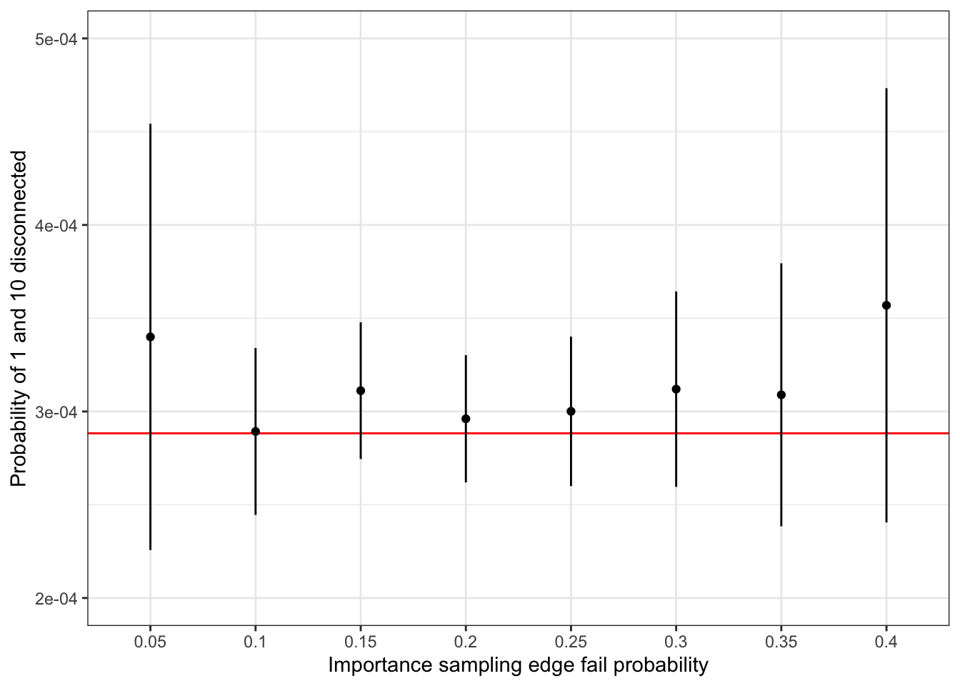
Figure 7.7: Confidence intervals for importance sampling estimates of network nodes 1 and 10 being disconnected under independent edge failures with probability 0.05. The red line is the true probability computed by complete enumeration.
7.3.1 Object oriented implementations
Implementations of algorithms that handle graphs and simulate graphs, as in the Monte Carlo
computations above, can benefit from using an object oriented approach. To
this end we first implement a so-called constructor, which is a function
that takes the adjacency matrix and the edge failure probability as arguments and
returns a list with class label network.
network <- function(A, p) {
  Aup <- A
  Aup[lower.tri(Aup)] <- 0
  ones <- which((Aup == 1))
  structure(
    list(
      A = A,
      Aup = Aup,
      ones = ones,
      p = p
    ),
    class = "network"
  )
}
We use the constructor function network() to construct and object of class
network for our specific adjacency matrix.
my_net <- network(A, p = 0.05)
str(my_net)
## List of 4
## $ A : num [1:10, 1:10] 0 1 0 1 1 0 0 0 0 0 ...
## $ Aup : num [1:10, 1:10] 0 0 0 0 0 0 0 0 0 0 ...
## $ ones: int [1:18] 11 22 31 41 44 52 53 63 66 73 ...
## $ p : num 0.05
## - attr(*, "class")= chr "network"
class(my_net)## [1] "network"The network object contains, in addition to A and p, two precomputed components:
the upper triangular part of the adjacency matrix; and the indices in that matrix
containing a 1.
The intention is then to write two methods for the network class. A method sim() that will
simulate a graph where some edges have failed, and a method failure() that will
estimate the probability of node 1 and 10 being disconnected by Monte Carlo
integration. To do so we need to define the two corresponding generic functions.
The method for simulation is then implemented as a function with name
sim.network.
sim.network <- function(x) {
  Aup <- x$Aup
  Aup[x$ones] <- sample(
    c(0, 1),
    length(x$ones),
    replace = TRUE,
    prob = c(x$p, 1 - x$p)
  )
  Aup
}
It is implemented using essentially the same implementation as sim_net()
except that Aup and p are extracted as components from the object x
instead of being arguments, and ones is extracted from x as well instead
of being computed. One could argue that the sim() method should return an object
of class network — that would be natural. However, then we need to call the
constructor with the full adjacency matrix, this will take some time and we do
not want to do that as a default. Thus we simply return the upper triangular
part of the adjacency matrix from sim().
The failure() method implements plain Monte Carlo integration as well
as importance sampling and returns a vector containing the estimate as
well as the 95% confidence interval. This implementation relies on the
already implemented functions discon() and weights().
failure.network <- function(x, n, p0 = NULL) {
  if (is.null(p0)) {
    # Plain Monte Carlo simulation
    tmp <- replicate(n, discon(sim(x)))
    mu_hat <- mean(tmp)
    se <- sqrt(mu_hat * (1 - mu_hat) / n)
  } else {
    # Importance sampling
    p <- x$p
    x$p <- p0
    tmp <- replicate(n, weights(x$Aup, sim(x), p0, p))
    se <- sd(tmp) / sqrt(n)
    mu_hat <- mean(tmp)
  }
  value <- mu_hat + 1.96 * se * c(-1, 0, 1)
  names(value) <- c("low", "estimate", "high")
  value
}
We test the implementation against the previously computed results.
set.seed(seed)  # Resetting seed
failure(my_net, n)
## low estimate high
## 0.000226 0.000340 0.000454
set.seed(seed)  # Resetting seed
failure(my_net, n, p0 = 0.2)
## low estimate high
## 0.000262 0.000296 0.000330We find that these are the same numbers as computed above, thus the object oriented implementation concurs with the non-object oriented on this example.
We benchmark the object oriented implementation to measure if there is
any runtime loss or improvement due to using objects.
One should expect a small computational overhead due to method dispatching,
that is, the procedure that R uses to look up the appropriate sim() method
for an object of class network. On the other hand, sim() does not recompute
ones every time.
bench::mark(
  sim_net = sim_net(Aup, 0.05),
  sim = sim(my_net),
  check = FALSE
)
## # A tibble: 2 × 6
## expression min median `itr/sec` mem_alloc `gc/sec`
## <bch:expr> <bch:tm> <bch:tm> <dbl> <bch:byt> <dbl>
## 1 sim_net 4.92µs 5.74µs 166059. 4.39KB 16.6
## 2 sim 4.8µs 5.66µs 170961. 1.02KB 34.2From the benchmark, the object oriented solution using sim() appears to be
a bit slower than sim_net() despite the latter recomputing ones, and
this can be explained by method dispatching taking of the order of 300 nanoseconds
during these benchmark computations.
Once we have taken an object oriented approach, we can also implement methods
for some standard generic functions, e.g. the print function. As this generic
function already exists, we simply need to implement a method for class network.
print.network <- function(x) {
  cat("#vertices: ", nrow(x$A), "\n")
  cat("#edges:", sum(x$Aup), "\n")
  cat("p = ", x$p, "\n")
}
my_net # Implicitly calls 'print'## #vertices: 10
## #edges: 18
## p = 0.05Our print method now prints out some summary information about the graph instead of just the raw list.
If you want to work more seriously with graphs, it is likely that you want to use an existing R package instead of reimplementing many graph algorithms. One of these packages is igraph, which also illustrates well an object oriented implementation of graph classes in R.
We start by constructing a new graph object from the adjacency matrix.
net <- graph_from_adjacency_matrix(A, mode = "undirected")
class(net)
## [1] "igraph"
net # Illustrates the print method for objects of class 'igraph'## IGRAPH 5b7e42a U--- 10 18 --
## + edges from 5b7e42a:
## [1] 1-- 2 1-- 4 1-- 5 2-- 3 2-- 6 3-- 6 3-- 7 3-- 8 3--10 4-- 5 4-- 8 5-- 8
## [13] 5-- 9 6-- 7 6--10 7--10 8-- 9 9--10The igraph package supports a vast number of graph computation, manipulation and visualization tools. We will here illustrate how igraph can be used to plot the graph and how we can implement a simulation method for objects of class igraph.
You can use plot(net), which will call the plot method for objects of class igraph.
But before doing so, we will specify a layout of the graph.
# You can generate a layout ...
net_layout <- layout_(net, nicely())
# ... or you can specify one yourself
net_layout <- matrix(
  c(-20,  1,
    -4,  3,
    -4,  1,
    -4, -1,
    -4, -3,
     4,  3,
     4,  1,
     4, -1,
     4, -3,
     20,  -1),
  ncol = 2, nrow = 10, byrow = TRUE)
The layout we have specified makes it easy to recognize the graph.
plot(net, layout = net_layout, asp = 0)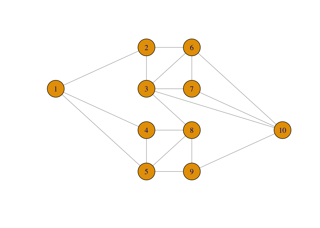
We then use two functions from the igraph package to implement simulation of
a new graph. We need gsize(), which gives the number of edges in the graph,
and we need delete_edges(), which removes edges from the graph. Otherwise
the simulation is still based on sample().
sim.igraph <- function(x, p) {
  deledges <- sample(
    c(TRUE, FALSE),
    gsize(x),        # 'gsize()' returns the number of edges
    replace = TRUE,
    prob = c(p, 1 - p)
  )
  delete_edges(x, which(deledges))
}
Note that this method is also called sim(), yet there is no conflict here with
the method for objects of class network because the generic sim() function
will delegate the call to the correct method based on the objects class label.
If we combine our new sim() method for igraphs with the plot method, we can
plot a simulated graph.
plot(sim(net, 0.25), layout = net_layout, asp = 0)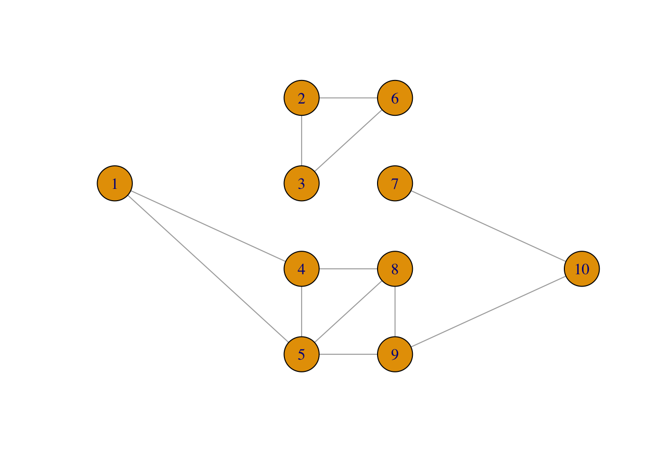
The implementation using igraph turns out to be a little slower than using
the matrix representation alone as in sim_net().
system.time(replicate(1e5, {sim(net, 0.05); NULL}))## user system elapsed
## 3.018 2.156 5.691One could also implement the function for testing if nodes 1 and 10 are
disconnected using the shortest_paths() function, but this is not faster
than the simple matrix multiplications used in discon() either. However, one
should be careful not to draw any general conclusions from this. Our graph is
admittedly a small toy example, and we implemented our solutions largely
to handle this particular graph.
7.4 Particle filters
We encountered some challenges in Section 7.2.2 when using importance sampling for computing a high-dimensional integral. Because we use a Monte Carlo average to approximate an integral, the Monte Carlo approximation can be quite poor if the function we average takes (relatively) large values occasionally. For importance sampling, this problem is often a consequence of the weights occasionally being large, and this happens when the proposal distribution deviates too much from the target distribution. For high-dimensional importance sampling, it can be quite difficult to find a proposal distribution that is sufficiently close to the target distribution.
In this section we introduce particle filters, which uses a form of sequentially adaptive proposals to alleviate the problem. Particle filters solve a collection of integration problems for the specific class of hidden Markov models, and they can be seen as a generalization of the Kalman filter.
7.4.1 Hidden Markov models
The hidden Markov model is a model of the random variables \((Y_1, Z_1), \ldots, (Y_N, Z_N)\) given by the following equations for \(k = 1, \ldots, N\):
\[\begin{align} Z_k &= F_k(Z_{k-1}, U_k) \tag{7.1} \\ Y_k &= G_k(Z_k, V_k), \tag{7.2} \end{align}\]
where \(U_1, \ldots, U_N\) and \(V_1, \ldots, V_N\) are independent and identically distributed random variables, and where \(F_k\) and \(G_k\) are some fixed maps. By convention, we let \(Z_0 = z_0\) take some fixed value. The equation (7.1) is a recursive update equation, which makes the \(X\)-s form a Markov chain. The equation (7.2) is known as the observation equation, and we generally suppose that we only observe the \(Y\)-s.
We introduce the notation \(Y_{1:k} = (Y_1, \ldots, Y_k)\) and similarly for \(Z_{1:k}\). Likewise, \(y_{1:k}\) and \(z_{1:k}\) denote specific observations of \(Y_{1:k}\) and \(Z_{1:k}\), respectively. Two standard problems that we want to solve are the computation of the following conditional expectations:
\[\begin{align} & \E\left( h(Z_k) \mid Y_{1:k} = y_{1:k} \right) \tag{7.3} \\ & \E\left( h(Z_k) \mid Y_{1:N} = y_{1:N} \right) \tag{7.4} \end{align}\]
where \(h\) is some real valued function. Computing the first conditional expectation (7.3) is known as a filtering problem, and the second (7.4) is known as a smoothing problem.
We first develop a bit of general theory that will show how the two conditional expectations can be expressed as (high-dimensional) integrals w.r.t. a distribution whose density is known up to a normalization constant. This suggests that we can use importance sampling with standardized weights to approximate the integrals. We show by example that the high-dimensional nature of the problem leads to similar problems as we encountered in Section 7.2.2. That is, weights will occasionally be very large, and the standardized weights will except for one or a few observations be very small. This is known as weight degeneracy, and it leads to poor performance of importance sampling. Particle filters are a solution to weight degeneracy.
7.4.2 Filtering and sequential importance sampling
We will for simplicity suppose that \(Z_k\) and \(Y_k\) are real valued random variables, and that the distributions of \(F_k(z, U_k)\) and \(G_k(z, V_k)\) have densities \(f_k(\cdot \mid z)\) and \(g_k(\cdot \mid z)\), respectively, w.r.t. Lebesgue measure. That is, the conditional distribution of \(Z_k | Z_{k-1} = z\) had density \(f_k(\cdot \mid z)\), and the conditional distribution of \(Y_k | Z_k = z\) has density \(g_k(\cdot \mid z)\). Then
\[\begin{align} f_{1:k}(z_{1:k}) & = f_1(z_1 \mid z_0) \cdot \ldots \cdot f_k(z_k \mid z_{k-1}) \\ & = f_{1:(k-1)}(z_{1:(t-1)}) \cdot f_k(z_k \mid z_{k-1}), \end{align}\]
is the density of \(Z_{0:i}\) w.r.t. Lebesgue measure in \(\mathbb{R}^i\). Likewise,
\[ g_{1:k}(y_{1:t} \mid z_{1:k}) = g_1(y_1 \mid z_1) g_2(y_2 \mid z_2) \ldots g_k(y_k \mid x_k) \]
is the conditional density of \(Y_{1:k}\) given \(Z_{1:k} = z_{1:k}\). It follows that the joint distribution of \((Y_1, Z_1), \ldots, (Y_k, Z_k)\) has density
\[ k_{1:k}(y_{1:k}, z_{1:k}) = g_{1:k}(y_{1:k} \mid z_{1:k}) f_{1:k}(z_{1:k}) \]
w.r.t. Lebesgue measure in \(\mathbb{R}^{2i}\). By Bayes’ theorem, the conditional density of \(Z_{1:k}\) given \(Y_{1:k} = y_{1:k}\) is
\[ f_{1:k}(z_{1:k} \mid y_{1:k}) = \frac{k_{1:k}(y_{1:k}, z_{1:k})}{g_{1:k}(y_{1:k})} \]
where the denominator is the marginal density of \(Y_{1:k}\), that is,
\[ g_{1:k}(y_{1:k}) = \int k_{1:k}(y_{1:k}, z_{1:k}) \mathrm{d}z_{1:k}. \]
Since
\[\begin{align*} \E\left( h(Z_k) \mid Y_{1:k} = y_{1:k} \right) & = \int h(z_k) f_{1:k}(z_{1:k} \mid y_{1:k}) \mathrm{d}z_{1:k} \\ & = \frac{\int h(z_k) k_{1:k}(y_{1:k}, z_{1:k}) \mathrm{d}z_{1:k}} {g_{1:k}(y_{1:k})} \\ & = \frac{\int h(z_k) g_{1:k}(y_{1:k} \mid z_{1:k}) f_{1:k}(z_{1:k}) \mathrm{d}z_{1:k}} {g_{1:k}(y_{1:k})}, \end{align*}\]
we see how the conditional expectation in the filtering problem can be expressed as an integral. The computation of the denomiator \(g_{1:k}(y_{1:k})\) is generally infeasible, thus we only know the target density up to a normalization constant.
If we use simulations from the Markov Chain itself as proposals, we identify the (unstandardized) weights from the integral above as
\[ w^*(Z_{1:k}) = g_{1:k}(y_{1:k} \mid Z_{1:k}) = w^*(Z_{1:(k-1)}) \cdot w^*(Z_{k}), \]
where \(w^*(Z_{k}) = g_k(y_k \mid Z_k)\). Since we can sample the Markov chain and compute the weights sequentially from \(Z_1\) to \(Z_k\), we call the corresponding algorithm sequential importance sampling.
With \(N\) i.i.d. observations \(Z_{1:N}^{(1)}, \ldots, Z_{1:N}^{(n)}\) of the Markov chain, we can approximate the conditional (filtering) expectation for any \(k\) as
\[ \E\left( h(Z_k) \mid Y_{1:k} = y_{1:k} \right) \approx \sum_{i=1}^N h(Z_k^{(i)}) w(Z_{1:k}^{(i)}) \]
where the standardized weights are
\[ w(Z_{1:k}^{(i)}) = \frac{w^*(Z_{1:k}^{(i)})}{\sum_{j=1}^N w^*(Z_{1:k}^{(j)})}. \]
Likewise, the conditional smoothing expectation can be approximated by
\[ \E\left( h(Z_k) \mid Y_{1:N} = y_{1:N} \right) \approx \sum_{i=1}^N h(Z_k^{(i)}) w(Z_{1:N}^{(i)}). \]
Example 7.1 We revisit the AR(1) model from Section 4.3 with the small notational difference that \(Z_k\) denotes the \(k\)-th unobserved variable instead of \(f_k\). Thus the update equation is linear and given as
\[ Z_k = \alpha Z_{k-1} + \tau U_k \]
where \(U_1, \ldots, U_N\) are i.i.d. standard Gaussian random variables, and \(\alpha \in \mathbb{R}\) and \(\tau > 0\) are fixed parameters. The observation equation is likewise linear and given as
\[ Y_k = Z_k + \sigma V_k \]
where \(V_1, \ldots, V_N\) are i.i.d. standard Gaussian random variables. We see that the AR(1) model is a special case of the general hidden Markov models considered in this section. In Section 4.3 we solved filtering and smoothing problems for the AR(1) model analytically, and we implemented the solution efficiently. Here we will use the AR(1) to illustrate the implementation of the sequential importance sampling algorithm, and we can the compare the results to those obtained by the analytic solution.
Since the conditional density of \(Y_k\) given \(Z_{k}\) is Gaussian we see that the unstandardized weights become
\[ w^*(Z_{k}) = \exp\left( - \frac{\left( y_k - Z_k \right)^2}{2 \sigma^2} \right). \]
7.5 Exercises
Exercise 7.1 Use that the univariate Gaussian density integrates to \(1\) to show that for any value of \(x_{k-1}\),
\[ \int \exp\left( - \frac{1}{2} (x_k - \alpha x_{k-1})^2 \right) \mathrm{d}x_k = (2 \pi)^{1/2}. \]
Use this to show by induction that
\[ \int \exp\left( - \frac{1}{2} \left( x_1^2 + \sum_{i=1}^p (x_k - \alpha x_{k-1})^2 \right) \right) \mathrm{d}x = (2 \pi)^{p/2}, \]
and argue that it implies
\[ \E\left( \exp\left(- \frac{1}{2} \sum_{i = 2}^p \alpha^2 X_{k-1}^2 - 2\alpha X_k X_{k-1} \right) \right) = 1. \]
if \(X \sim \mathcal{N}(0, I_p)\).