9 Numerical optimization
The main application of numerical optimization in statistics is computation of parameter estimates. Typically by maximizing the likelihood function or by maximizing or minimizing another estimation criterion. The focus of this chapter is on optimization algorithms for (penalized) maximum likelihood estimation. Out of tradition we formulate all results and algorithms in terms of minimization and not maximization.
The generic optimization problem considered is the minimization of a function \(H: \Theta \to \mathbb{R}\) for \(\Theta \subseteq \mathbb{R}^p\) an open set and \(H\) twice differentiable. In applications we might consider \(H = -\ell\), the negative log-likelihood function, or \(H = -\ell + J\), where \(J : \Theta \to \mathbb{R}\) is a penalty function, likewise twice differentiable, that does not depend upon data.
Most statistical optimization problems share a common structure that we should pay attention to. Given data points \(y_1, \ldots, y_N\) the negative log-likelihood
\[ -\ell(\theta) = - \sum_{i=1}^N \log(f_{\theta}(y_i)) \]
is a sum over the data, and the more data we have the more computationally demanding it is to evaluate \(-\ell\) and its derivatives. There are exceptions, though, when a sufficient statistic can be computed upfront, but generally we must expect runtime to grow with data size.
We should also note that blindly pursuing the global maximum of the likelihood can lead us astray if our model is not well behaved. Kiefer (1978) demonstrated that for the Gaussian mixture model introduced in Section 8.3.1, the likelihood (with unknown variance parameters) is unbounded. Yet Kiefer showed that for \(H = - \ell\) there exists a consistent sequence of solutions to the equation \(\nabla H(\theta) = 0\) as \(N \to \infty\). That is, the unknown parameters can be estimated consistently by computing stationary points of \(H\)—even if these do not globally minimize \(H\). In situations where \(H\) is not convex and where \(H\) may be unbounded below, it might still be possible to compute a good parameter estimate as a local minimizer. So even if we phrase the objective as a global optimization problem, we may be equally interested in local minima or even just stationary points; solutions to \(\nabla H(\theta) = 0\).
Optimization is a computational technique used in statistics for adapting models to data—but the minimizer of \(H\) for a particular data set is not intrinsically interesting. It is typically unnecessary to compute a (local) minimizer to high numerical precision. If the numerical error is already orders of magnitudes smaller than the statistical uncertainty of the parameter estimate being computed, further optimization makes no relevant difference. Rather than computing a single numerically accurate minimizer we should use our computational resources to explore many models and many starting values for the numerical optimizers, and we should assess the various model fits and quantify the model and parameter uncertainties.
For the generic minimization problem considered in this chapter, the practical
challenge when implementing algorithms in R is typically to implement efficient
evaluation of \(H\) and its derivatives. In particular, efficient evaluations of
the negative log-likelihood, \(-\ell\). Several choices of standard optimization algorithms are possible and
some are already implemented and available in R. For many practical purposes the
BFGS-algorithms, as implemented via optim(), work well and require only the
computation of gradients. It is, of course, paramount that \(H\) and \(\nabla H\)
are correctly implemented, and efficiency of the algorithms is largely
determined by the efficiency of the implementation of \(H\) and \(\nabla H\) as well
as by the choice of parametrization.
9.1 Peppered moths
We revisit in this section the peppered moth example from Section 8.2.2,
where we implemented the log-likelihood for general multinomial distributions
with collapsing of categories, and where we
computed the maximum-likelihood estimate via
optim(). We used the default Nelder-Mead algorithm, which does not require
derivatives. In this section we implement the gradient as well and
illustrate how to optimize a function via optim() using the conjugate
gradient algorithm and the BFGS-algorithm.
From the expression for the log-likelihood in (8.1) it follows that the gradient equals
\[ \nabla \ell(\theta) = \sum_{j = 1}^{K_0} \frac{ n_j }{ M(p(\theta))_j}\nabla M(p(\theta))_j = \sum_{j = 1}^{K_0} \sum_{k \in A_j} \frac{ n_j}{ M(p(\theta))_j} \nabla p_k(\theta). \]
Letting \(j(k)\) be defined by \(k \in A_{j(k)}\) we see that the gradient can also be written as
\[ \nabla \ell(\theta) = \sum_{k=1}^K \frac{n_{j(k)}}{ M(p(\theta))_{j(k)}} \nabla p_k(\theta) = \tilde{\mathbf{x}}(\theta) \mathrm{D}p(\theta), \]
where \(\mathrm{D}p(\theta)\) is the Jacobian of the parametrization \(\theta \mapsto p(\theta)\), and \(\tilde{\mathbf{x}}(\theta)\) is the vector with
\[ \tilde{\mathbf{x}}(\theta)_k = \frac{ n_{j(k)}}{M(p(\theta))_{j(k)}}. \]
We first recall the implementation of the general log-likelihood function
in the multinomial model with cell collapsing before implementing the
gradient based on the formula above. The gradient takes the Jacobian
of the parametrization, \(Dp\), as an argument. If the parameters are out of
bounds, it returns a vector of NAs.
mult_collapse <- function(ny, group) {
  as.vector(tapply(ny, group, sum))
}

neg_loglik_mult <- function(par, ny, prob, group, ...) {
  p <- prob(par)
  if (is.null(p)) return(Inf)
  - sum(ny * log(mult_collapse(p, group)))
}

grad_neg_loglik_mult <- function(par, ny, prob, Dprob, group) {
  p <- prob(par)
  if (is.null(p)) return(rep(NA, length(par)))
  - (ny[group] / mult_collapse(p, group)[group]) %*% Dprob(par)
}
For the specific example of peppered moths we recall how to implement the parametrization of the multinomial probabilities.
prob_pep <- function(p) {
  p[3] <- 1 - p[1] - p[2]

  out_of_bounds <-
    p[1] > 1 || p[1] < 0 || p[2] > 1 || p[2] < 0 || p[3] < 0
  if (out_of_bounds) return(NULL)

  c(p[1]^2, 2 * p[1] * p[2], 2 * p[1] * p[3],
    p[2]^2, 2 * p[2] * p[3], p[3]^2
  )
}
Finally, we also need to implement the problem specific Jacobian for the peppered moths example.
Dprob_pep <- function(p) {
  p[3] <- 1 - p[1] - p[2]
  matrix(
    c(2 * p[1],             0,
      2 * p[2],             2 * p[1],
      2 * p[3] - 2 * p[1], -2 * p[1],
      0,                    2 * p[2],
      -2 * p[2],            2 * p[3] - 2 * p[2],
      -2 * p[3],           -2 * p[3]),
    ncol = 2, nrow = 6, byrow = TRUE)
}
We can then use the conjugate gradient algorithm, say, to compute the maximum-likelihood estimate.
optim(c(0.3, 0.3), neg_loglik_mult, grad_neg_loglik_mult,
  ny = c(85, 196, 341),
  prob = prob_pep,
  Dprob = Dprob_pep,
  group = c(1, 1, 1, 2, 2, 3),
  method = "CG"
)
## $par
## [1] 0.07084 0.18874
##
## $value
## [1] 600.5
##
## $counts
## function gradient
## 131 25
##
## $convergence
## [1] 0
##
## $message
## NULLNOTE ON THE ... in the implementation of neg_loglike_mult().
The peppered moth example is very simple.
The log-likelihood can easily be computed, and we used this
problem to illustrate ways of implementing a
likelihood in R and how to use optim() to maximize it.
The first likelihood implementation in Section 8.2.2
is very problem specific
while the second is more abstract and general, and we used the same general and abstract
approach to implement the gradient above. The gradient could then
be used for other optimization algorithms, still using optim(), such as
conjugate gradient. In fact, we can use conjugate gradient without
computing and implementing the gradient.
optim(c(0.3, 0.3), neg_loglik_mult,
  ny = c(85, 196, 341),
  prob = prob_pep,
  group = c(1, 1, 1, 2, 2, 3),
  method = "CG"
)
## $par
## [1] 0.07084 0.18874
##
## $value
## [1] 600.5
##
## $counts
## function gradient
## 110 15
##
## $convergence
## [1] 0
##
## $message
## NULLIf we do not implement a gradient, a numerical gradient is used by optim().
This can result in a slower algorithm than if the gradient is implemented, but
more seriously, in can result in convergence problems. This is because there is
a subtle tradeoff between numerical accuracy and accuracy of the finite
difference approximation used to approximate the gradient. We did not experience
convergence problems in the example above, but if one encounters such problems
a possible solution is to change the parscale or fnscale entries
in the control list argument to optim().
Chapter 10 revisits the peppered moth example and use it to illustrate the EM algorithm for computing the maximum-likelihood estimate. It is important to understand that the EM algorithm does not rely on the ability to compute the (log-)likelihood—or the gradient of the (log-)likelihood for that matter. In some applications of the EM algorithm the computation of the likelihood is challenging or even impossible, in which case most standard optimization algorithms will not be directly applicable.
9.2 Algorithms and convergence
In the subsequent sections of this chapter we will investigate the implementation of several standard optimization algorithms—including the conjugate gradient algorithm used for the peppered moth example in the previous section. In this section we develop a minimal theoretical framework for presenting and analyzing optimization algorithms and their convergence. This establishes a rudimentary theoretical understanding of sufficient conditions for convergence, but equally importantly it provides us with a precise framework for quantifying and measuring convergence of algorithms in practice.
A numerical optimization algorithm computes from an initial value \(\theta_0 \in \Theta\) a sequence \(\theta_1, \theta_2, \ldots \in \Theta\). We could hope for
\[ \theta_n \rightarrow \theta_{\infty} = \argmin_{\theta} H(\theta) \]
for \(n \to \infty\), but less can typically be guaranteed. First, the global minimizer may not exist or it may not be unique, in which case the convergence itself is undefined or ambiguous. Second, \(\theta_n\) can in general only be shown to converge to a local minimizer if anything. Third, \(\theta_n\) may not converge, even if \(H(\theta_n)\) converges to a local minimum.
To discuss properties of optimization algorithms in greater detail we need ways to quantify, analyze and monitor their convergence. This can be done in terms of \(\theta_n\), \(H(\theta_n)\) or \(\nabla H(\theta_n)\). Focusing on \(H(\theta_n)\) we say that an algorithm is a descent algorithm if
\[ H(\theta_0) \geq H(\theta_1) \geq H(\theta_2) \geq \ldots. \]
If all inequalities are sharp (except if some \(\theta_i\) is a local minimizer), the algorithm is called a strict descent algorithm. The sequence \(H(\theta_n)\) is convergent for any descent algorithm if \(H\) is bounded from below, e.g., if the level set
\[ \mathrm{lev}(\theta_0) = \{\theta \in \Theta \mid H(\theta) \leq H(\theta_0)\} \]
is compact. However, even for a strict descent algorithm, \(H(\theta_n)\) may descent in smaller and smaller steps toward a limit that is not a (local) minimum. A good optimization algorithm needs to guarantee more than descent—it needs to guarantee sufficient descent in each step.
Many algorithms can be phrased as
\[ \theta_n = \Phi(\theta_{n-1}) \]
for a map \(\Phi : \Theta \to \Theta\). When \(\Phi\) is continuous and \(\theta_n \rightarrow \theta_{\infty}\) it follows that
\[ \Phi(\theta_n) \rightarrow \Phi(\theta_{\infty}). \]
Since \(\Phi(\theta_n) = \theta_{n+1} \rightarrow \theta_{\infty}\) we see that
\[ \Phi(\theta_{\infty}) = \theta_{\infty}. \]
That is, \(\theta_{\infty}\) is a fixed point of \(\Phi\). If \(\theta_n\) is not convergent, any accumulation point of \(\theta_n\) will still be a fixed point of \(\Phi\). Thus we can search for potential accumulation points by searching for fixed points of the map \(\Phi: \Theta \to \Theta\).
Mathematics is full of fixed point theorems that: i) give conditions under which a map has a fixed point; and ii) in some cases guarantee that the iterates \(\Phi^{\circ n}(\theta_0)\) converge to a fixed point. The most prominent result is Banach’s fixed point theorem. It states that if \(\Phi\) is a contraction, that is,
\[ \| \Phi(\theta) - \Phi(\theta')\| \leq c \|\theta - \theta'\| \]
for a constant \(c \in [0,1)\) (using any norm), then \(\Phi\) has a unique fixed point and \(\theta_n = \Phi^{\circ n}(\theta_0)\) converges to that fixed point for any starting point \(\theta_0 \in \Theta\).
We will show how a simple gradient descent algorithm can be analyzed—both as a descent algorithm and through Banach’s fixed point theorem. This will demonstrate basic proof techniques as well as typical conditions on \(H\) that can give convergence results for optimization algorithms. We will only scratch the surface here with the intention that it can motivate the algorithms introduced in subsequent sections and chapters as well as empirical techniques for practical assessment of convergence.
Indeed, theory rarely provides us with sharp quantitative results on the rate of convergence and we will need computational techniques to monitor and measure convergence of algorithms in practice. Otherwise we cannot compare the efficiency of different algorithms.
9.2.1 Gradient descent
We will assume in this section that \(\Theta = \mathbb{R}^p\). This will simplify the analysis a bit, but with minor modifications it can be generalized to the case where \(\Theta\) is open and convex.
Suppose that \(D^2H(\theta)\) has numerical radius uniformly bounded by \(L\), that is,
\[ |\gamma^T D^2H(\theta) \gamma| \leq L \|\gamma\|_2^2 \]
for all \(\theta \in \Theta\) and \(\gamma \in \mathbb{R}^p\). The gradient descent algorithm with a fixed step length \(1/(L + 1)\) is given by
\[\begin{align} \theta_{n} & = \theta_{n-1} - \frac{1}{L + 1} \nabla H(\theta_{n-1}). \tag{9.1} \end{align}\]
Fixing \(n\) there is by Taylor’s theorem a \(\tilde{\theta} = \alpha \theta_{n} + (1- \alpha)\theta_{n-1}\) (where \(\alpha \in [0,1]\)) on the line between \(\theta_n\) and \(\theta_{n-1}\) such that
\[\begin{align*} H(\theta_n) & = H(\theta_{n-1}) - \frac{1}{L+1} \|\nabla H(\theta_{n-1})\|_2^2 + \\ & \qquad \frac{1}{(L+1)^2} \nabla H(\theta_{n-1})^T D^2H(\tilde{\theta}) \nabla H(\theta_{n-1}) \\ & \leq H(\theta_{n-1}) - \frac{1}{L+1} \|\nabla H(\theta_{n-1})\|_2^2 + \frac{L}{(L+1)^2} \|\nabla H(\theta_{n-1})\|_2^2 \\ & = H(\theta_{n-1}) - \frac{1}{(L+1)^2} \|\nabla H(\theta_{n-1})\|_2^2. \end{align*}\]
This shows that \(H(\theta_n) \leq H(\theta_{n-1})\), and if \(\theta_{n-1}\) is not a stationary point, \(H(\theta_n) < H(\theta_{n-1})\). That is, the algorithm is a descent algorithm, and unless it hits a stationary point it is a strict descent algorithm.
It furthermore follows that
\[\begin{align*} H(\theta_n) & = (H(\theta_n) - H(\theta_{n-1})) + (H(\theta_{n-1}) - H(\theta_{n-2})) + ... \\ & \qquad + (H(\theta_1) - H(\theta_0)) + H(\theta_0) \\ & \leq H(\theta_0) - \frac{1}{(L + 1)^2} \sum_{k=1}^n \|\nabla H(\theta_{k-1})\|_2^2. \end{align*}\]
If \(H\) is bounded below, \(\sum_{k=1}^{\infty} \|\nabla H(\theta_{k-1})\|_2^2 < \infty\) and hence
\[ \|\nabla H(\theta_{n})\|_2 \rightarrow 0 \]
for \(n \to \infty\). For any accumulation point, \(\theta_{\infty}\), of the sequence \(\theta_n\), it follows by continuity of \(\nabla H\) that
\[ \nabla H(\theta_{\infty}) = 0, \]
and \(\theta_{\infty}\) is a stationary point. If \(H\) has a unique stationary point in \(\mathrm{lev}(\theta_0)\), \(\theta_{\infty}\) is a (local) minimizer, and
\[ \theta_n \rightarrow \theta_{\infty} \]
for \(n \to \infty\).
The gradient descent algorithm (9.1) is given by the map
\[ \Phi_{\nabla}(\theta) = \theta - \frac{1}{L + 1} \nabla H(\theta). \]
The gradient descent map, \(\Phi_{\nabla}\), has \(\theta\) as fixed point if and only if
\[ \nabla H(\theta) = 0, \]
that is, if and only if \(\theta\) is a stationary point.
We will show that \(\Phi_{\nabla}\) is a contraction on \(\Theta\) under the assumption that the eigenvalues of the (symmetric) matrix \(D^2H(\theta)\) for all \(\theta \in \Theta\) are contained in an interval \([l, L]\) with \(0 < l \leq L\). If \(\theta, \theta' \in \Theta\) we find by Taylor’s theorem that
\[ \nabla H(\theta) = \nabla H(\theta') + D^2H(\tilde{\theta})(\theta - \theta') \]
for some \(\tilde{\theta}\) on the line between \(\theta\) and \(\theta'\). For the gradient descent map this gives that
\[\begin{align*} \|\Phi_{\nabla}(\theta) - \Phi_{\nabla}(\theta')\|_2 & = \left\|\theta - \theta' - \frac{1}{L+1}\left(\nabla H(\theta) - \nabla H(\theta')\right)\right\|_2 \\ & = \left\|\theta - \theta' - \frac{1}{L+1}\left( D^2H(\tilde{\theta})(\theta - \theta')\right)\right\|_2 \\ & = \left\|\left(I - \frac{1}{L+1} D^2H(\tilde{\theta}) \right) (\theta - \theta')\right\|_2 \\ & \leq \left(1 - \frac{l}{L + 1}\right) \|\theta - \theta'\|_2, \end{align*}\]
since the eigenvalues of \(I - \frac{1}{L+1} D^2H(\tilde{\theta})\) are all between \(1 - L/(L + 1)\) and \(1 - l/(L+1)\). This shows that \(\Phi_{\nabla}\) is a contraction for the \(2\)-norm with \(c = 1 - l/(L + 1) < 1\). From Banach’s fixed point theorem it follows that there is a unique stationary point, \(\theta_{\infty}\), and \(\theta_n \rightarrow \theta_{\infty}\). Since \(D^2H(\theta_{\infty})\) is positive definite, \(\theta_{\infty}\) is a (global) minimizer.
To summarize, if \(D^2H(\theta)\) has uniformly bounded numerical radius, and if \(H\) has a unique stationary point \(\theta_{\infty}\) in the compact set \(\mathrm{lev}(\theta_0)\), then the gradient descent algorithm is a strict descent algorithm that converges toward that (local) minimizer \(\theta_{\infty}.\) The fixed step length was key to this analysis. The upper bound on the numerical radius of \(D^2H(\theta)\) guarantees descent with a fixed step length, and the fixed step length then guarantees sufficient descent.
When the eigenvalues of \(D^2H(\theta)\) are in \([l, L]\) for \(0 < l \leq L\), \(H\) is a strongly convex function with a unique global minimizer \(\theta_{\infty}\) and all level sets \(\mathrm{lev}(\theta_0)\) compact. Convergence can then also be established via Banach’s fixed point theorem. The constant \(c = 1 - l/(L + 1) = 1 - \kappa^{-1}\) with \(\kappa = (L + 1) / l\) then quantifies the rate of the convergence, as will be discussed in greater detail in the next section. The constant \(\kappa\) is an upper bound on the conditioning number of the matrix \(D^2H(\theta)\) uniformly in \(\theta\), and a large value of \(\kappa\) means that \(c\) is close to 1 and the convergence can be slow. A large conditioning number for the second derivative indicates that the graph of \(H\) looks like a narrow ravine, in which case we can expect the gradient descent algorithm to be slow.
9.2.2 Convergence rate
When \(\theta_n = \Phi^{\circ n}(\theta_0)\) for a contraction \(\Phi\), Banach’s fixed point theorem tells us that there is a unique fixed point \(\theta_{\infty}.\) That \(\Phi\) is a contraction further implies that
\[ \|\theta_n - \theta_{\infty}\| = \|\Phi(\theta_{n-1}) - \theta_{\infty}\| \leq c \|\theta_{n-1} - \theta_{\infty}\| \leq c^n \|\theta_0 - \theta_{\infty}\|. \]
That is, \(\|\theta_n - \theta_{\infty}\| \to 0\) with at least geometric rate \(c < 1\).
In the numerical optimization literature, convergence at a geometric rate is known as linear convergence (the number of correct digits increases linearly with the number of iterations), and a linearly convergent algorithm is often quantified in terms of its asymptotic convergence rate.
Definition 9.1 Let \((\theta_n)_{n \geq 1}\) be a convergent sequence in \(\mathbb{R}^p\) with limit \(\theta_{\infty}\). Let \(\| \cdot \|\) be a norm on \(\mathbb{R}^p\). We say that the convergence is linear if
\[ \limsup_{n \to \infty} \frac{\|\theta_{n} - \theta_{\infty}\|}{\|\theta_{n-1} - \theta_{\infty}\|} = r \]
for some \(r \in (0, 1)\), in which case \(r\) is called the asymptotic rate.
Convergence of an algorithm can be faster or slower than linear. If
\[ \limsup_{n \to \infty} \frac{\|\theta_{n} - \theta_{\infty}\|}{\|\theta_{n-1} - \theta_{\infty}\|} = 1 \]
we say that the convergence is sublinear, and if
\[ \limsup_{n \to \infty} \frac{\|\theta_{n} - \theta_{\infty}\|}{\|\theta_{n-1} - \theta_{\infty}\|} = 0 \]
we say that the convergence is superlinear. There is also a refined notion of convergence order for superlinearly convergent algorithms that more precisely describes the convergence.
For a contraction, \(\theta_n = \Phi^{\circ n}(\theta_0)\) converges linearly or superlinearly. If it converges linearly, the asymptotic rate is bounded by \(c\), but this is a global constant and may be pessimistic. The following lemma provides a local upper bound on the asymptotic rate in terms of the derivative of \(\Phi\) in the limit \(\theta_{\infty}\).
Lemma 9.1 Let \(\Phi : \mathbb{R}^p \to \mathbb{R}^p\) be twice continuously differentiable. If \(\theta_n = \Phi^{\circ n}(\theta_0)\) converges linearly toward a fixed point \(\theta_{\infty}\) of \(\Phi\) then
\[ r_{\max} = \sup_{\gamma: \|\gamma \| = 1} \|D \Phi(\theta_{\infty}) \gamma\| \]
is an upper bound on the asymptotic rate.
Proof. By Taylor’s theorem,
\[\begin{align*} \theta_{n} = \theta_{\infty} + D \Phi(\theta_{\infty})(\theta_{n-1} - \theta_{\infty}) + o(\|\theta_{n-1} - \theta_{\infty}\|_2). \end{align*}\]
Rearranging yields
\[\begin{align*} \limsup_{n \to \infty} \frac{\| \theta_{n} - \theta_{\infty}\|}{\| \theta_{n-1} - \theta_{\infty}\|} & = \limsup_{n \to \infty} \frac{\| D \Phi(\theta_{\infty})(\theta_{n-1} - \theta_{\infty})\|}{\| \theta_{n-1} - \theta_{\infty}\|} \\ & = \limsup_{n \to \infty} \| D \Phi(\theta_{\infty})\left(\frac{\theta_{n-1} - \theta_{\infty}}{\| \theta_{n-1} - \theta_{\infty}\|} \right)\| \\ & \leq r_{\max}. \end{align*}\]
Note that it is possible that \(r_{\max} \geq 1\) even if the convergence is linear, in which case \(r_{\max}\) is a useless upper bound. Moreover, the actual rate can depend on the starting point \(\theta_0\), and even when \(r_{\max} < 1\) it only quantifies the worst case convergence rate.
To estimate the actual convergence rate, note that linear convergence with rate \(r\) implies that for any \(\delta > 0\)
\[ \| \theta_n - \theta_{\infty} \| \leq (r + \delta) \| \theta_{n-1} - \theta_{\infty} \| \leq \ldots \leq (r + \delta)^{n - n_0} \| \theta_{n_0} - \theta_{\infty} \| \]
\(n \geq n_0\) with \(n_0\) sufficiently large (depending on \(\delta\)). That is,
\[ \log \|\theta_{n} - \theta_{\infty}\| \leq n \log(r + \delta) + d, \]
for \(n \geq n_0\). In practice, we run the algorithm for \(M\) iterations, so that \(\theta_M = \theta_{\infty}\) up to computer precision, and we plot \(\log \|\theta_{n} - \theta_{M}\|\) as a function of \(n\). The decay should be approximately linear for \(n \geq n_0\) for some \(n_0\), in which case the slope is about \(\log(r) < 0\), which can then be estimated by least squares. A slower-than-linear or faster-than-linear decay indicate that the algorithm converges sublinearly or superlinearly, respectively.
It is, of course, possible to quantify convergence in terms of the sequences \(H(\theta_n)\) and \(\nabla H(\theta_n)\) instead. For a descent algorithm with \(H(\theta_n) \rightarrow H(\theta_\infty)\) linearly for \(n \to \infty\), we can plot
\[ \log(H(\theta_n) - H(\theta_M)) \]
as a function of \(n\), and use least squares to estimate the asymptotic rate of convergence of \(H(\theta_n)\).
Using \(\nabla H(\theta_n)\) to quantify convergence is particularly appealing as we know that the limit is \(0\). This also means that we can monitor its convergence while the algorithm is running and not only after it has converged. If \(\nabla H(\theta_n)\) converges linearly in the norm \(\|\cdot\|\), that is,
\[ \limsup_{n \to \infty} \frac{\|\nabla H(\theta_n)\|}{\|\nabla H(\theta_{n-1})\|} = r, \]
we have for any \(\delta > 0\) that
\[ \log \|\nabla H(\theta_n)\| \leq n \log(r + \delta) + d \]
for \(n \geq n_0\) and \(n_0\) sufficiently large. Again, least squares can be used to estimate the asymptotic rate of convergence of \(\|\nabla H(\theta_n)\|\).
The concepts of linear convergence and asymptotic rate are, unfortunately, not independent of the norm used, nor does linear convergence of \(\theta_n\) in \(\|\cdot\|\) imply linear convergence of \(H(\theta_n)\) or \(\|\nabla H(\theta_n)\|\). We can show, though, that if \(\theta_n\) converges linearly in the norm \(\| \cdot \|\), the other two sequences converge linearly along an arithmetic subsequence. Similarly, it can be shown that in any other norm than \(\| \cdot \|\), \(\theta_n\) is also linearly convergent along an arithmetic subsequence.
Theorem 9.1 Suppose that \(H\) is three times continuously differentiable with \(\nabla H (\theta_{\infty}) = 0\) and \(D^2 H(\theta_{\infty})\) positive definite. If \(\theta_n\) converges linearly toward \(\theta_{\infty}\) in any norm then for some \(k \geq 1\), the subsequences \(H(\theta_{nk})\) and \(\|\nabla H(\theta_{nk})\|\) converge linearly toward \(H(\theta_{\infty})\) and \(0\), respectively.
Proof. Let \(G = D^2 H(\theta_{\infty})\) and \(g_n = \theta_n - \theta_{\infty}\). Since \(G\) is positive definite it defines a norm, and since all norms on \(\mathbb{R}^p\) are equivalent there are constants \(a, b > 0\) such that
\[ a \| x \|^2 \leq x^T G x \leq b \| x \|^2. \]
By Taylor’s theorem,
\[ H(\theta_{(n + 1)k}) - H(\theta_{\infty}) = g_{(n + 1)k}^T G g_{(n + 1)k} + o(\|g_{(n + 1)k}\|^2). \]
From this,
\[\begin{align*} \limsup_{n \to \infty} \frac{H(\theta_{(n + 1)k}) - H(\theta_{\infty})}{H(\theta_{nk}) - H(\theta_{\infty})} & = \limsup_{n \to \infty} \frac{g_{(n + 1)k}^T G g_{(n + 1)k}}{g_{nk}^T G g_{nk}} \\ & \leq \limsup_{n \to \infty} \frac{b \| g_{(n + 1)k}\|^2}{a \| g_{nk}\|^2} = \frac{b}{a} r^{2k} \end{align*}\]
where \(r \in (0, 1)\) is the asymptotic rate of \(\theta_n \to \theta_{\infty}\). By choosing \(k\) sufficiently large, the right hand side above is strictly smaller than 1, which gives an upper bound on the rate along the subsequence \(H(\theta_{nk})\). A similar argument gives a lower bound strictly larger than 0, which shows that the convergence is not superlinear.
Using Taylor’s theorem on \(\nabla H(\theta_{nk})\) yields a similar proof for the subsequence \(\|\nabla H(\theta_{nk})\|\)—with \(G\) replaced by \(G^2\) in the bounds.
The bounds in the proof are often pessimistic since \(g_n\) and \(g_{n+1}\) can point in completely different directions. Exercise ?? shows, however, that if \(\theta_n\) approaches \(\theta_{\infty}\) nicely along a fixed direction (making \(g_n\) and \(g_{n+1}\) almost collinear), \(H(\theta_n)\) as well as \(\|\nabla H(\theta_n)\|\) inherit linear convergence from \(\theta_n\) and even with the same rate.
All rates discussed hithereto are per iteration, which is natural when investigating a single algorithm. However, different algorithms may spend different amounts of time per iteration, and it does not make sense to make a comparison of per iteration rates across different algorithms. We therefore need to be able to convert between per iteration and per time unit rates. If one iteration takes \(\delta\) time units (seconds, say) the per time unit rate is
\[ r^{1/\delta}. \]
If \(t_n\) denotes the runtime of \(n\) iterations, we could estimate \(\delta\) as \(t_M / M\) for \(M\) sufficiently large.
We will throughout systematically investigate convergence as a function of time \(t_n\) instead of iterations \(n\), and we will estimate rates per time unit directly by least squares regression on \(t_n\) instead of \(n\).
9.2.3 Stopping criteria
One important practical question remains unanswered even if we understand the theoretical convergence properties of an algorithm well and have good methods for measuring its convergence rates. No algorithm can run for an infinite number of iterations, thus all algorithms need a criterion for when to stop, but the choice of an appropriate stopping criterion is notoriously difficult. We present four of the most commonly used criteria and discuss benefits and deficits for each of them.
Maximum number of iterations: Stop when
\[ n = M \]
for a fixed maximum number of iterations \(M\). This is arguably the simplest criterion, but, obviously, reaching a maximum number of iterations provides no evidence in itself that \(H(\theta_M)\) is sufficiently close to a (local) minimum. For a specific problem we could from experience know of a sufficiently large \(M\) so that the algorithm has typically converged after \(M\) iterations, but the most important use of this criterion is in combination with another criterion so that it works as a safeguard against an infinite loop.
The other three stopping criteria all depend on choosing a tolerance parameter \(\varepsilon > 0\), which will play different roles in the three criteria. The three criteria can be used individually and in combinations, but unfortunately neither of them nor their combination provide convergence guarantees. It is nevertheless common say that an algorithm “has converged” when the stopping criterion is satisfied, but since none of the criteria are sufficient for convergence this can be a bit misleading.
Small relative change: Stop when
\[ \|\theta_n - \theta_{n-1}\| \leq \varepsilon(\|\theta_n\| + \varepsilon). \]
The idea is that when \(\theta_n \approx \theta_{n-1}\) the sequence has approximately reached the limit \(\theta_{\infty}\) and we can stop. It is possible to use an absolute criterion such as \(\|\theta_n - \theta_{n-1}\| < \varepsilon\), but then the criterion would be sensitive to a rescaling of the parameters. Thus fixing a reasonable tolerance parameter across many problems makes more sense for the relative then the absolute criterion. The main reason for adding \(\varepsilon\) on the right hand size is to make the criterion well behaved even if \(\|\theta_n\|\) is close to zero.
The main benefit of this criterion is that it does not require evaluations of the objective function. Some algorithms, such as the EM algorithm, do not need to evaluate the objective function, and it may even be difficult to do so. In those cases this criterion can be used. The main deficit is that a single iteration with little change in the parameter can happen for many reasons besides convergence, and it does not imply that neither \(\|\theta_n - \theta_{\infty}\|\) nor \(H(\theta_{n}) - H(\theta_{\infty})\) are small.
Small relative descent: Stop when
\[ H(\theta_{n-1}) - H(\theta_n) \leq \varepsilon (|H(\theta_n)| + \varepsilon). \]
This criterion only makes sense if the algorithm is a descent algorithm. As discussed above, an absolute criterion would be sensitive to rescaling of the objective function, and the added \(\varepsilon\) on the right hand side is to ensure a reasonable behavior if \(H(\theta_n)\) is close to zero.
This criterion is natural for descent algorithms; we stop when the algorithm does not decrease the value of the objective function sufficiently. The use of a relative criterion makes is possible to choose a tolerance parameter that works reasonably well for many problems. A conventional choice is \(\varepsilon \approx 10^{-8}\) (and often chosen as the square root of the machine epsilon), though the theoretical support for this choice is weak. The deficit of the algorithm is as for the criterion above: a small descent does not imply that \(H(\theta_{n}) - H(\theta_{\infty})\) is small, and it could happen if the algorithm enters a part of \(\Theta\) where \(H\) is very flat, say.
Small gradient: Stop when
\[ \|\nabla H(\theta_n)\| \leq \varepsilon. \]
This criterion directly measures if \(\theta_n\) is close to being a stationary point (and not if \(\theta_n\) is close to a stationary point). A small value of \(\|\nabla H(\theta_n)\|\) is still no guarantee that \(\|\theta_n - \theta_{\infty}\|\) or \(H(\theta_{n}) - H(\theta_{\infty})\) are small. The criterion also requires the computation of the gradient. In addition, different norms can be used, and if different coordinates of the gradient are of different orders of magnitude this should be reflected by the norm. Alternatively, the parameters should be rescaled.
Neither of the four criteria above gives a theoretical convergence guarantee in terms of how close \(H(\theta_{n})\) is to \(H(\theta_{\infty})\) or how close \(\theta_n\) is to \(\theta_{\infty}\). In some special cases it is, however, possible to make stronger statements. If \(H\) is , there is a constant \(C\) such that
\[ \|\theta_n - \theta_{\infty}\| \leq C \|\nabla H(\theta_n)\|, \]
and the small gradient stopping criterion will, actually, imply that \(\theta_n\) is close to \(\theta_{\infty}\)—if \(\epsilon\) is small relative to \(C\). Another approach is based on a lower envelope. If there is a continuous function \(\tilde{H}\) satisfying \(H(\theta_{\infty}) = \tilde{H}(\theta_{\infty})\) and
\[ H(\theta_{\infty}) \geq \tilde{H}(\theta) \]
for all \(\theta \in \Theta\) (or just in \(\mathrm{lev}(\theta_0)\) for a descent algorithm) then
\[ 0 \leq H(\theta_{n}) - H(\theta_{\infty}) \leq H(\theta_{n}) - \tilde{H}(\theta_{n}), \]
and the right hand side directly quantifies convergence. Convex duality theory gives for many convex optimization problems such a function, \(\tilde{H}\), and in those cases a convergence criterion based on \(H(\theta_{n}) - \tilde{H}(\theta_{n})\) actually comes with a theoretical guarantee on how close we are to the minimum. We will not pursue the necessary convex duality theory here, but it is useful to know that in some cases we can do better than the ad hoc criteria above.
9.3 Descent direction algorithms
The negative gradient of \(H\) in \(\theta\) is the direction of steepest descent. Since the goal is to minimize \(H\), it is natural to move away from \(\theta\) in the direction of \(-\nabla H(\theta)\). However, other directions than the negative gradient can also be suitable descent directions.
Definition 9.2 A descent direction in \(\theta\) is a vector \(\rho \in \mathbb{R}^p\) such that
\[ \nabla H(\theta)^T \rho < 0. \]
When \(\theta\) is not a stationary point,
\[ \nabla H(\theta)^T(-\nabla H(\theta)) = - \| \nabla H(\theta)^T \|_2^2 < 0 \]
and \(-\nabla H(\theta)^T\) is a descent direction in \(\theta\) according to the definition.
Given \(\theta_n\) and a descent direction \(\rho_n\) in \(\theta_n\) we can define
\[ \theta_{n+1} = \theta_n + \gamma \rho_n \]
for a suitably chosen \(\gamma > 0\). By Taylor’s theorem
\[ H(\theta_{n+1}) = H(\theta_n) + \gamma \nabla H(\theta_n) \rho_n + o(\gamma), \]
which means that
\[ H(\theta_{n+1}) < H(\theta_n) \]
if \(\gamma\) is small enough.
One strategy for choosing \(\gamma\) is to minimize the univariate function
\[ \gamma \mapsto H(\theta_n + \gamma \rho_n), \]
which is an example of a line search method. Such a minimization would give the maximal possible descent in the direction \(\rho_n\), and as we have argued, if \(\rho_n\) is a descent direction, a minimizer \(\gamma > 0\) guarantees descent of \(H\). However, unless the minimization can be done analytically it is often computationally too expensive. Less will also do, and as shown in Section 9.2.1, if the Hessian has uniformly bounded numerical radius it is possible to fix one (sufficiently small) step length that will guarantee descent.
9.3.1 Line search
We consider algorithms of the form
\[ \theta_{n+1} = \theta_n + \gamma_{n} \rho_n \]
starting in \(\theta_n\) and with \(\rho_n\) a descent direction in \(\theta_n\). The step lengths, \(\gamma_n\), should be chosen so as to give sufficient descent in each iteration.
The function \(h(\gamma) = H(\theta_{n} + \gamma \rho_{n})\) is a univariate and differentiable function,
\[ h : [0,\infty) \to \mathbb{R}, \]
that gives the value of \(H\) in the descent direction \(\rho_n\). We find that
\[ h'(\gamma) = \nabla H(\theta_{n} + \gamma \rho_{n})^T \rho_{n}, \]
and the maximal descent in direction \(\rho_n\) can be found by solving \(h'(\gamma) = 0\) for \(\gamma\). As mentioned above, less will do. First note that
\[ h'(0) = \nabla H(\theta_{n})^T \rho_{n} < 0, \]
so \(h\) has a negative slope in \(0\). It descents in a sufficiently small interval \([0, \varepsilon)\), and it is even true that for any \(c \in (0, 1)\) there is an \(\varepsilon > 0\) such that
\[ h(\gamma) \leq h(0) + c \gamma h'(0) \]
for \(\gamma \in [0, \varepsilon)\). We note that this inequality can be checked easily for any given \(\gamma > 0\), and is known as the sufficient descent condition. Sufficient descent is not enough in itself as the step length could be arbitrarily small, and the algorithm could effectively get stuck.
To prevent too small steps we can enforce another condition. Very close to \(0\), \(h\) will have almost the same slope, \(h'(0)\), as it has in \(0\). If we therefore require that the slope in \(\gamma\) should be larger than \(\tilde{c} h'(0)\) for some \(\tilde{c} \in (0, 1)\), \(\gamma\) is forced away from \(0\). This is known as the curvature condition.
The combined conditions on \(\gamma\),
\[ h(\gamma) \leq h(0) + c \gamma h'(0) \]
for a \(c \in (0, 1)\) and
\[ h'(\gamma) \geq \tilde{c} h'(0) \]
for a \(\tilde{c} \in (c, 1)\) are known collectively as the Wolfe conditions. It can be shown that if \(h\) is bounded below there exists a step length satisfying the Wolfe conditions (Lemma 3.1 in Nocedal and Wright (2006)).
Even when choosing \(\gamma_{n}\) to fulfill the Wolfe conditions there is no guarantee that \(\theta_n\) will converge let alone converge toward a global minimizer. The best we can hope for in general is that
\[ \|\nabla H(\theta_n)\|_2 \rightarrow 0 \]
for \(n \to \infty\), and this will happen under some relatively weak conditions on \(H\) (Theorem 3.2 Nocedal and Wright (2006)) under the assumption that
\[ \frac{\nabla H(\theta_n)^T \rho_n}{\|\nabla H(\theta_n)\|_2 \| \rho_n\|_2} \leq - \delta < 0. \]
That is, the angle between the descent direction and the gradient should be uniformly bounded away from \(90^{\circ}\).
A practical way of searching for a step length is via backtracking. Choosing a \(\gamma_0\) and a constant \(d \in (0, 1)\) we can search through the sequence of step lengths
\[ \gamma_0, d \gamma_0, d^2 \gamma_0, d^3 \gamma_0, \ldots \]
and stop the first time we find a step length satisfying the Wolfe conditions.
Using backtracking, we can actually dispense of the curvature condition and simply check the sufficient descent condition
\[ H(\theta_{n} + d^k \gamma_0 \rho_{n}) \leq H(\theta_n) + cd^k \gamma_0 \nabla H(\theta_{n})^T \rho_{n} \]
for \(c \in (0, 1)\). The implementation of backtracking requires the choice of the three parameters: \(\gamma_0 > 0\), \(d \in (0, 1)\) and \(c \in (0, 1)\). A good choice depends quite a lot on the algorithm used for choosing the descent direction, but choosing \(c\) too close to 1 can make the algorithm take too small steps, and taking \(d\) too small can likewise generate small step lengths. Thus \(d = 0.8\) or \(d = 0.9\) and \(c = 0.1\) or even smaller are sensible choices. For some algorithms, like the Newton algorithm to be dealt with below, there is a natural choice of \(\gamma_0 = 1\). But for other algorithms a good choice depends crucially on the scale of the parameters, and there is then no general advice on choosing \(\gamma_0\).
9.3.2 Gradient descent
We implement gradient descent with backtracking below as the function grad_desc().
For gradient descent, the sufficient descent condition amounts to
choosing the smallest \(k \geq 0\) such that
\[ H(\theta_{n} - d^k \gamma_0 \nabla H(\theta_{n})) \leq H(\theta_n) - cd^k \gamma_0 \|\nabla H(\theta_{n})\|_2^2. \]
The grad_desc() function takes the starting point, \(\theta_0\), the objective function,
\(H\), and its gradient, \(\nabla H\), as arguments. The four parameters \(d\), \(c\), \(\gamma_0\) and
\(\varepsilon\) that control the algorithm can also be specified as additional arguments,
but are given some reasonable default values. The implementation uses the squared norm of
the gradient as a stopping criterion, but it also has a maximum number of
iterations as a safeguard. If the maximum number is reached, a
warning is printed.
Finally, we include a callback argument (the cb argument).
If a function is passed to this argument, it will be evaluated in each iteration
of the algorithm. This gives us the possibility of logging or
printing values of variables during evaluation, which can be highly useful
for understanding the inner workings of the algorithm. Monitoring or logging
intermediate values during the evaluation of code is referred to as
tracing.
grad_desc <- function(
  par,
  H,
  gr,
  d = 0.8,
  c = 0.1,
  gamma0 = 0.01,
  epsilon = 1e-4,
  maxit = 1000,
  cb = NULL
) {
  for (n in 1:maxit) {
    value <- H(par)
    grad <- gr(par)
    h_prime <- sum(grad^2)
    if (!is.null(cb)) cb()
    # Convergence criterion based on gradient norm
    if (h_prime <= epsilon) break
    gamma <- gamma0
    # Proposed descent step
    par1 <- par - gamma * grad
    # Backtracking while descent is insufficient
    while (H(par1) > value - c * gamma * h_prime) {
      gamma <- d * gamma
      par1 <- par - gamma * grad
    }
    par <- par1
  }
  if (n == maxit) {
    warning("Maximum number, ", maxit, ", of iterations reached")
  }
  par
}
We will use the Poisson regression example to illustrate the use of gradient descent and other optimization algorithms, and we need to implement functions in R for computing the negative log-likelihood and its gradient.
The implementation below uses a function factory to produce a list containing a parameter vector, the negative log-likelihood function and its gradient. We anticipate that for the Newton algorithm in Section 9.4 we also need an implementation of the Hessian, which is thus included here as well.
We will exploit the model.matrix() function to construct the model matrix
from the data via a formula, and the sufficient statistic is also
computed. The implementations use linear algebra and vectorized computations
relying on access to the model matrix and the sufficient statistics in
their enclosing environment.
poisson_model <- function(form, data, response) {
  X <- model.matrix(form, data)
  y <- data[[response]]
  # The computation of t(X) %*% y is more efficiently done by
  # crossprod(X,y). Use the function drop() to drop the dim attribute
  # and turn a matrix with one column into a vector
  t_map <- drop(crossprod(X, y))
  N <- nrow(X)
  p <- ncol(X)

  H <- function(beta)
    drop(sum(exp(X %*% beta)) - beta %*% t_map) / N

  grad <- function(beta)
    (drop(crossprod(X, exp(X %*% beta))) - t_map) / N

  Hessian <- function(beta)
    crossprod(X, drop(exp(X %*% beta)) * X) / N

  list(par = rep(0, p), H = H, grad = grad, Hessian = Hessian)
}
We choose to normalize the log-likelihood by the number of observations \(N\) (the number of rows in the model matrix). This does have a tiny computational cost, but the resulting numerical values become less dependent upon \(N\), which makes it easier to choose sensible default values of various parameters for the numerical optimization algorithms. Gradient descent is very slow for the large Poisson model with individual store effects, so we consider only the simple model with two parameters.
veg_pois <- poisson_model(
  ~ log(normalSale),
  CSwR::vegetables,
  response = "sale"
)
pois_gd <- grad_desc(veg_pois$par, veg_pois$H, veg_pois$grad)The gradient descent implementation is tested by comparing the minimizer to
the estimated parameters as computed by glm().
rbind(pois_glm = coefficients(pois_model_null), pois_gd)## (Intercept) log(normalSale)
## pois_glm 1.461 0.9216
## pois_gd 1.460 0.9219We get the same result up to the first two decimals. The convergence criterion on our gradient descent algorithm was quite loose (\(\varepsilon = 10^{-4}\), which means that the norm of the gradient is smaller than \(10^{-2}\) when the algorithm stops). This choice of \(\varepsilon\) in combination with \(\gamma_0 = 0.01\) implies that the algorithm stops when the gradient is so small that the changes are at most of norm \(10^{-4}\).
Comparing the resulting values of the negative log-likelihood shows agreement
up to the first five decimals, but we notice that the negative log-likelihood
for the parameters fitted using glm() is just slightly smaller.
veg_pois$H(coefficients(pois_model_null))
veg_pois$H(pois_gd)
## [1] -124.406827879897
## [1] -124.406825325047To investigate what actually went on inside the gradient descent
algorithm we will use the callback argument to trace the internals
of a call to grad_desc(). The tracer() function from the CSwR package
can be used to construct a tracer object with a tracer() function that we can pass as the callback
argument. The tracer object and its tracer() function work by storing
information in the enclosing environment of tracer(). When used as
the callback argument to, e.g., grad_desc() the tracer() function will look up
variables in the evaluation environment of grad_desc(), store them and
print them if requested, and store runtime information as well.
When grad_desc() has returned, the trace information can be accessed
via the summary() method for the tracer object. The tracer objects
and their tracer() function should not be confused with the trace()
function from the R base package, but the tracer object’s tracer() function
can be passed as the tracer argument to trace() to interactively
inject tracing code into any R function. Here, the tracer objects will
only be used together with a callback argument.
We use the tracer object with our gradient descent implementation and print trace information every 50th iteration.
gd_tracer <- CSwR::tracer(c("value", "h_prime", "gamma"), Delta = 50)
pois_gd <- grad_desc(
  veg_pois$par,
  veg_pois$H,
  veg_pois$grad,
  cb = gd_tracer$tracer
)
## n = 1: value = 1; h_prime = 14269; gamma = NA;
## n = 50: value = -123.9; h_prime = 15.46; gamma = 0.004096;
## n = 100: value = -124.3; h_prime = 3.134; gamma = 0.00512;
## n = 150: value = -124.4; h_prime = 0.6014; gamma = 0.00512;
## n = 200: value = -124.4; h_prime = 0.09806; gamma = 0.00512;
## n = 250: value = -124.4; h_prime = 0.01097; gamma = 0.00512;
## n = 300: value = -124.4; h_prime = 0.002376; gamma = 0.00512;
## n = 350: value = -124.4; h_prime = 0.0002165; gamma = 0.004096;We see that the gradient descent algorithm runs for a little more than 350 iterations, and we can observe how the value of the negative log-likelihood is descending. We can also see that the step length \(\gamma\) bounces between \(0.004096 = 0.8^4 \times 0.01\) and \(0.00512 = 0.8^3 \times 0.01\), thus the backtracking takes 3 to 4 iterations to find a step length with sufficient descent.
The printed trace does not reveal the runtime information. The runtime is measured for each iteration of the algorithm and the cumulative runtime is of greater interest. This information can be computed and inspected after the algorithm has converged, and it is returned by the summary method for tracer objects.
##      value   h_prime    gamma   .time
## 372 -124.4 1.126e-04 0.005120 0.02216
## 373 -124.4 1.219e-04 0.005120 0.02222
## 374 -124.4 1.324e-04 0.005120 0.02228
## 375 -124.4 1.442e-04 0.005120 0.02234
## 376 -124.4 1.575e-04 0.005120 0.02240
## 377 -124.4 7.601e-05 0.004096 0.02247
The trace information is stored in a list. The summary method transforms the trace information into a data frame with one row per iteration. We can also access individual entries of the list of trace information via subsetting.
gd_tracer[377] ## $value
## [1] -124.4
##
## $h_prime
## [1] 7.601e-05
##
## $gamma
## [1] 0.004096
##
## $.time
## [1] 6.548e-05
Figure 9.1: Gradient norm (left) and value of the negative log-likelihood (right) above the limit value \(H(\theta_{\infty})\). The straight line is fitted to the data points except the first ten using least squares, and the rate is computed from this estimate and reported per ms.
9.3.3 Conjugate gradients
The gradient direction is not the best descent direction. It is too local, and convergence can be quite slow. One of the better algorithms that is still a first order algorithm (using only gradient information) is the nonlinear conjugate gradient algorithm. In the Fletcher–Reeves version of the algorithm the descent direction is initialized as the negative gradient \(\rho_0 = - \nabla H(\theta_{0})\) and then updated as
\[ \rho_{n} = - \nabla H(\theta_{n}) + \frac{\|\nabla H(\theta_n)\|_2^2}{\|\nabla H(\theta_{n-1})\|_2^2} \rho_{n-1}. \]
That is, the descent direction, \(\rho_{n}\), is the negative gradient but modified according to the previous descent direction. There is plenty of opportunity to vary the prefactor of \(\rho_{n-1}\), and the one presented here is what makes it the Fletcher–Reeves version. Other versions go by the names of their inventors such as Polak–Ribière or Hestenes–Stiefel.
In fact, \(\rho_{n}\) need not be a descent direction unless we put some restrictions on the step lengths. One possibility is to require that the step length \(\gamma_{n}\) satisfies the strong curvature condition
\[ |h'(\gamma)| = |\nabla H(\theta_n + \gamma \rho_n)^T \rho_n | \leq \tilde{c} |\nabla H(\theta_n)^T \rho_n| = \tilde{c} |h'(0)| \]
for a \(\tilde{c} < \frac{1}{2}\). Then \(\rho_{n + 1}\) can be shown to be a descent direction if \(\rho_{n}\) is.
We implement the conjugate gradient method in a slightly different way. Instead of introducing the more advanced curvature condition, we simply reset the algorithm to use the gradient direction in any case where a non-descent direction has been chosen. Resets of descent direction every \(p\)-th iteration is recommended anyway for the nonlinear conjugate gradient algorithm.
conj_grad <- function(
  par,
  H,
  gr,
  d = 0.8,
  c = 0.1,
  gamma0 = 0.05,
  epsilon = 1e-10,
  maxit = 10000,
  cb = NULL
) {
  p <- length(par)
  m <- 1
  rho0 <- numeric(p)
  for(n in 1:maxit) {
    value <- H(par)
    grad <- gr(par)
    grad_norm_sq <- sum(grad^2)
    if(!is.null(cb)) cb()
    if(grad_norm_sq <= epsilon) break
    gamma <- gamma0
    # Descent direction
    rho <- - grad + grad_norm_sq * rho0
    h_prime <- drop(t(grad) %*% rho)
    # Reset to gradient if m > p or rho is not a descent direction
    if(m > p || h_prime >= 0) {
      rho <- - grad
      h_prime <- - grad_norm_sq
      m <- 1
    }
    par1 <- par + gamma * rho
    # Backtracking
    while(H(par1) > value + c * gamma * h_prime) {
      gamma <- d * gamma
      par1 <- par + gamma * rho
    }
    rho0 <- rho / grad_norm_sq
    par <- par1
    m <- m + 1
  }
  if(n == maxit)
    warning("Maximum number, ", maxit, ", of iterations reached")
  par
}
cg_tracer <- CSwR::tracer(c("value", "gamma", "grad_norm_sq"), Delta = 25)
pois_cg <- conj_grad(
  veg_pois$par,
  veg_pois$H,
  veg_pois$grad,
  cb = cg_tracer$tracer
)
## n = 1: value = 1; gamma = NA; grad_norm_sq = 14269;
## n = 25: value = -124.29; gamma = 0.004295; grad_norm_sq = 16.782;
## n = 50: value = -124.4; gamma = 0.02048; grad_norm_sq = 0.27642;
## n = 75: value = -124.41; gamma = 0.004295; grad_norm_sq = 0.0061342;
## n = 100: value = -124.41; gamma = 0.02048; grad_norm_sq = 0.0001485;
## n = 125: value = -124.41; gamma = 0.004295; grad_norm_sq = 2.7515e-06;
## n = 150: value = -124.41; gamma = 0.0256; grad_norm_sq = 1.4018e-07;
## n = 175: value = -124.41; gamma = 0.004295; grad_norm_sq = 1.472e-09;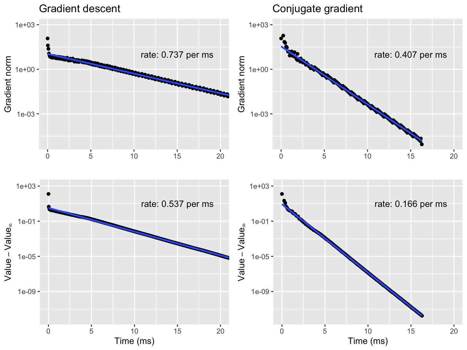
Figure 9.2: Gradient norms (top) and negative log-likelihoods (bottom) for gradient descent (left) and conjugate gradient (right).
This algorithm is fast enough to fit the large Poisson regression model.
veg_pois_large <- poisson_model(
  ~ store + log(normalSale) - 1,
  CSwR::vegetables,
  response = "sale"
)
cg_tracer <- CSwR::tracer(c("value", "gamma", "grad_norm_sq"), Delta = 400)
pois_cg <- conj_grad(
  veg_pois_large$par,
  veg_pois_large$H,
  veg_pois_large$grad,
  cb = cg_tracer$tracer
)
## n = 1: value = 1; gamma = NA; grad_norm_sq = 12737;
## n = 400: value = -128.4; gamma = 0.004295; grad_norm_sq = 1.4219;
## n = 800: value = -128.57; gamma = 0.0083886; grad_norm_sq = 0.088079;
## n = 1200: value = -128.59; gamma = 0.0014074; grad_norm_sq = 0.025125;
## n = 1600: value = -128.59; gamma = 0.0014074; grad_norm_sq = 2.4173e-06;
## n = 2000: value = -128.59; gamma = 0.004295; grad_norm_sq = 1.3028e-05;
## n = 2400: value = -128.59; gamma = 0.0011259; grad_norm_sq = 3.9599e-07;## value gamma grad_norm_sq .time
## 2745 -128.6 0.050000 7.939e-10 9.800
## 2746 -128.6 0.020480 7.174e-09 9.802
## 2747 -128.6 0.001126 1.096e-08 9.807
## 2748 -128.6 0.016384 6.082e-09 9.809
## 2749 -128.6 0.002199 8.983e-10 9.814
## 2750 -128.6 0.002199 9.958e-11 9.818Using optim() with the conjugate gradient method.
bench::bench_time(
  pois_optim_cg <- optim(
    veg_pois_large$par,
    veg_pois_large$H,
    veg_pois_large$grad,
    method = "CG",
    control = list(maxit = 10000)
  )
)
## process real
## 6.7s 6.64s
pois_optim_cg[c("value", "counts")]## $value
## [1] -128.6
##
## $counts
## function gradient
## 11586 49529.4 Newton-type algorithms
The Newton algorithm is similar to gradient descent except that the gradient is replaced by
\[ \rho_n = - D^2 H(\theta_n)^{-1} \nabla H(\theta_n) \]
as a descent direction.
The Newton algorithm is typically much more efficient than gradient descent per iteration and will converge in few iterations. However, the storage of the \(p \times p\) Hessian, its computation, and the solution of the equation to compute \(\rho_n\) all scale like \(p^2\) and this can make the algorithm useless for large \(p\).
The standard Newton algorithm for a general objective function is implemented
in R via the function nlm(). Note that its interface differs from optim()
in terms of the order and type of the arguments, and the gradient
(and Hessian) are passed to nlm() as attributes to the objective function
rather than as arguments to nlm() itself. For non-linear least squares
problems the nls() function (with yet another interface) should be
considered.
We implement a standard Newton algorithm with backtracking below, which includes a
callback option allowing us to trace the internals of the algorithm. It is a
straightforward modification of grad_desc() where we add the Hessian to the argument
list and change the descent direction.
newton <- function(
  par,
  H,
  gr,
  hess,
  d = 0.8,
  c = 0.1,
  gamma0 = 1,
  epsilon = 1e-10,
  maxit = 50,
  cb = NULL
) {
  for(n in 1:maxit) {
    value <- H(par)
    grad <- gr(par)
    grad_norm_sq <- sum(grad^2)
    if(!is.null(cb)) cb()
    if(grad_norm_sq <= epsilon) break
    Hessian <- hess(par)
    rho <- - drop(solve(Hessian, grad))
    gamma <- gamma0
    par1 <- par + gamma * rho
    h_prime <- t(grad) %*% rho
    while(H(par1) > value +  c * gamma * h_prime) {
      gamma <- d * gamma
      par1 <- par + gamma * rho
    }
    par <- par1
  }
  if(n == maxit)
    warning("Maximum number, ", maxit, ", of iterations reached")
  par
}
There exists a variety of alternatives to the Newton algorithm that replace the Hessian by another matrix that can be easier to compute and update. That is, the descent directions are of the form
\[ \rho_n = - B_n \nabla H(\theta_n) \]
for a \(p \times p\) matrix \(B_n\). With \(B_n = D^2 H(\theta_n)^{-1}\) we get the standard Newton algorithm. Whether \(\rho_n\) is actually a descent direction depends on \(B_n\). A sufficient condition is that \(B_n\) is a positive definite matrix.
9.4.1 Poisson regression
We reconsider the Poisson regression model, pois_model, from Section
8.4, which was also considered in Section 9.3.3.
There we used conjugate gradient descent to estimate the 353 parameters.
Recall that the veg_pois_large list contains all the functions needed to
run the Newton algorithm—including the Hessian matrix.
newton_tracer <- CSwR::tracer(
  c("value", "gamma", "grad_norm_sq"),
  Delta = 0
)
pois_newton <- newton(
  veg_pois_large$par,
  veg_pois_large$H,
  veg_pois_large$grad,
  veg_pois_large$Hessian,
  cb = newton_tracer$tracer
)
We compare the resulting parameter estimates to those in pois_model,
computed using glm.fit().
range(pois_newton - coefficients(pois_model))## [1] -4.979e-10 1.299e-06The differences between all parameters are very small. We can also compare the corresponding values of the objective function, and we include in this comparison the value found using conjugate gradient.
rbind(
  pois_cg = veg_pois_large$H(pois_cg),
  pois_newton = veg_pois_large$H(pois_newton),
  pois_glm = veg_pois_large$H(coefficients(pois_model))
)
## [,1]
## pois_cg -128.58945047360265335
## pois_newton -128.58945047446982812
## pois_glm -128.58945047447090815We see that these values are also extremely close with the first 12 digits identical.
We finally study the trace information from running our Newton algorithm.
summary(newton_tracer)## value gamma grad_norm_sq .time
## 1 1.00 NA 1.274e+04 0.0000
## 2 -14.83 0.02252 4.475e+04 0.1686
## 3 -64.82 0.26214 8.476e+04 0.3324
## 4 -111.34 1.00000 1.144e+04 0.4982
## 5 -124.25 1.00000 9.723e+02 0.6549
## 6 -127.71 1.00000 8.048e+01 0.8117
## 7 -128.50 1.00000 5.133e+00 0.9684
## 8 -128.59 1.00000 9.585e-02 1.1242
## 9 -128.59 1.00000 7.168e-05 1.2807
## 10 -128.59 1.00000 4.645e-11 1.4503We note the relatively few iterations used (10 in this case) to reach the stringent stopping criterion that the squared gradient norm is less than \(10^{-10}\). This took less than \(2\) seconds. Compare this to the \(12\)–\(15\) seconds it took the conjugate gradient algorithm to reach a similarly accurate value of the minimizer. By inspecting the trace information (not shown) for conjugate gradient it turns out that after the first \(1\)–\(1.5\) second (about 250 iterations) it reached roughly the same accuracy as Newton did in its first \(7\) iterations. Thereafter, conjugate gradient spend the rest of the time improving the accuracy slowly while Newton in just \(3\) additional iterations converged to a very accurate minimizer. This is a characteristic behavior of Newton, which has superlinear (in fact, quadratic) convergence.
It is natural to ask if the R function glm.fit(), which also uses a Newton
algorithm (without backtracking), is faster than our implementation.
env_pois <- environment(veg_pois_large$H)
bench::bench_time(
  glm.fit(env_pois$X, env_pois$y, family = poisson())
)
## process real
## 329ms 324msUsing glm.fit() is about a factor five faster on this example than
our Newton algorithm—but we should always be very careful when comparing
the runtimes of two different optimization algorithms. In this case they
have achieved about the same numerical precision, and by the comparison
above of the optimized value of the objective function,
the faster glm.fit() even obtained the smallest negative
log-likelihood of the two.
9.4.2 Quasi-Newton algorithms
We turn to other descent direction algorithms that are more efficient than gradient descent by choosing the descent direction in a more clever way but less computationally demanding than the Newton algorithm that requires the computation of the full Hessian in each iteration.
We will only consider the application of the BFGS algorithm via the
implementation in the R function optim().
bench::bench_time(
  pois_bfgs <- optim(
    veg_pois_large$par,
    veg_pois_large$H,
    veg_pois_large$grad,
    method = "BFGS",
    control = list(maxit = 10000)
  )
)
## process real
## 183ms 180ms
range(pois_bfgs$par - coefficients(pois_model))## [1] -0.00955 0.08481
pois_bfgs[c("value", "counts")]## $value
## [1] -128.6
##
## $counts
## function gradient
## 158 1489.4.3 Sparsity
One of the benefits of the implementations of \(H\) and its derivatives as well as of the descent algorithms is that they can exploit sparsity of \(\mathbf{X}\) almost for free. The implementations have not done that in previous computations, because \(\mathbf{X}\) has been stored as a dense matrix. In reality, \(\mathbf{X}\) is a very sparse matrix (the vast majority of the matrix entries are zero), and if we convert it into a sparse matrix, all the matrix-vector products will be more runtime efficient. Sparse matrices are implemented in the R package Matrix.
## [1] "dgCMatrix"
## attr(,"package")
## [1] "Matrix"
Without changing any other code, we get an immediate
runtime improvement using, e.g., optim() and the BFGS algorithm.
bench::bench_time(
  pois_bfgs_sparse <- optim(
    veg_pois_large$par,
    veg_pois_large$H,
    veg_pois_large$grad,
    method = "BFGS",
    control = list(maxit = 10000)
  )
)
## process real
## 60.4ms 59.4msWe should in real applications avoid constructing a dense intermediate
model matrix as a step toward constructing a sparse model matrix. This
is possible by constructing the sparse model matrix directly using
a function from the R package MatrixModels. Ideally, we should reimplement
pois_model() to support an option for using sparse matrices, but
to focus on the runtime benefits of sparse matrices, we simply
change the matrix in the appropriate environment directly.
env_pois$X <- MatrixModels::model.Matrix(
  ~ store + log(normalSale) - 1,
  data = CSwR::vegetables,
  sparse = TRUE
)
class(env_pois$X)
## [1] "dsparseModelMatrix"
## attr(,"package")
## [1] "MatrixModels"The Newton implementation benefits enormously from using sparse matrices because the bottleneck is the computation of the Hessian.
newton_tracer <- CSwR::tracer(c("value", "h_prime", "gamma"), Delta = 0)
  pois_newton <- newton(
  veg_pois_large$par,
  veg_pois_large$H,
  veg_pois_large$grad,
  veg_pois_large$Hessian,
  cb = newton_tracer$tracer
)
summary(newton_tracer)
## value h_prime gamma .time
## 1 1.00 NA NA 0.000000
## 2 -14.83 -4.141e+03 0.02252 0.002484
## 3 -64.82 -4.030e+02 0.26214 0.003977
## 4 -111.34 -7.636e+01 1.00000 0.004671
## 5 -124.25 -2.104e+01 1.00000 0.005349
## 6 -127.71 -5.652e+00 1.00000 0.006048
## 7 -128.50 -1.333e+00 1.00000 0.006819
## 8 -128.59 -1.647e-01 1.00000 0.007583
## 9 -128.59 -4.160e-03 1.00000 0.008260
## 10 -128.59 -3.289e-06 1.00000 0.008921To summarize the runtimes we have measured for the Poisson regression example, we found that the conjugate gradient algorithms took of the order of 10 seconds to converge. The Newton-type algorithms in this section were faster and took between 0.3 and 1.7 seconds to converge. The use of sparse matrices reduced the runtime of the quasi-Newton algorithm BFGS by a factor 3, but it reduced the runtime of the Newton algorithm by a factor 150 to about 0.009 seconds. One could be concerned that the construction of the sparse model matrix takes more time (which we did not measure), but if measured it turns out that for this example it takes about the same time to construct the dense model matrix as it takes to construct the sparse one.
Runtime efficiency is not the only argument for using sparse matrices as they are also more memory efficient. It is memory (and time) inefficient to use dense intermediates, and for truly large scale problems impossible. Using sparse model matrices for regression models allows us to work with larger models that have more variables, more factor levels and more observations than if we use dense model matrices. For the Poisson regression model the memory used by either representation can be found.
object.size(env_pois$X)
object.size(as.matrix(env_pois$X))
## Sparse matrix memory usage:
## 123440 bytes
## Dense matrix memory usage:
## 3103728 bytesWe see that the dense matrix uses around a factor 30 more memory than the
sparse representation. In this case it means using around 3 MB for storing the
dense matrix instead of around 100 kB, which won’t be a problem
on a contemporary computer. However, going from using 3 GB for
storing a matrix to using 100 Mb could be the difference between
not being able to work with the matrix on a standard laptop to
running the computations with no problems. Using model.Matrix() makes
it possible to construct sparse model matrices directly and avoid
all dense intermediates.
The function glm4() from the MatrixModels package for fitting regression models,
can exploit sparse model matrices direction, and can
thus be useful in cases where your model matrix becomes very large but sparse.
There are two main applications where the model matrix becomes sparse.
When you model the response using one or more factors, and possibly their
interactions, the model matrix will become particularly sparse if
the factors have many levels. Another case is when you model the response
via basis expansions of quantitative predictors and use basis functions
with local support. The B-splines form an important example of such a basis
with local support that results in a sparse model matrix.
9.5 Misc.
If \(\Phi\) is just nonexpansive (the constant \(c\) above is one), this is no longer true, but replacing \(\Phi\) by \(\alpha \Phi + (1 - \alpha) I\) for \(\alpha \in (0,1)\) we get Krasnoselskii-Mann iterates of the form
\[ \theta_n = \alpha \Phi(\theta_{n-1}) + (1 - \alpha) \theta_{n-1} \]
that will converge to a fixed point of \(\Phi\) provided it has one.
Banach’s fixed point theorem implies a convergence that is at least as fast as linear convergence with asymptotic rate \(c\). Moreover, if \(\Phi\) is just a contraction for \(n \geq n_0\) for some \(n_0\), then for \(n \geq n_0\)
\[ \|\theta_{n + 1} - \theta_{n}\| \leq c \| \theta_{n} - \theta_{n-1}\|. \]
The convergence may be superlinear, but if it is linear, the rate is bounded by \(c\). To indicate if \(\Phi\) is asymptotically a contraction, we can introduce
\[ R_n = \frac{\|\theta_{n + 1} - \theta_{n}\|}{\|\theta_{n} - \theta_{n- 1}\|} \]
and monitor its behavior as \(n \to \infty\). The constant
\[ r = \limsup_{n \to \infty} R_n \]
is then asymptotically the smallest possible contraction constant. If convergence is sublinear and \(R_n \to 1\) the sequence is called logarithmically convergent (by definition), while \(r \in (0,1)\) is an indication of linear convergence with rate \(r\), and \(r = 0\) is an indication of superlinear convergence.
In practice, we can plot the ratio \(R_n\) as the algorithm is running, and use \(R_n\) as an estimate of the rate \(r\) for large \(n\). However, this can be a quite unstable method for estimating the rate.
Finally, it is also possible to estimate the order \(q\) as well as the rate \(r\) by using that \[\log \|\theta_{n} - \theta_{N}\| \approx q \log \|\theta_{n-1} - \theta_{N}\| + \log(r)\] for \(n \geq n_0\). We can estimate \(q\) and \(\log(r)\) by fitting a linear function by least squares to these log-log transformed norms of errors.
Iteration, fixed points, convergence criteria. Ref to Nonlinear Parameter Optimization Using R Tools.